---

List of Sources:

• Young et al., 2020¹
• Image generated by WordPress AI

---

Table of Contents:

1. Angular Velocity and Acceleration (Young et al., 2020)
   1. Angular Velocity
   2. Angular Velocity as a Vector
   3. Angular Acceleration
   4. Angular Acceleration as a Vector
2. Rotation with Constant Angular Acceleration (Young et al., 2020)
   1. Comparing Angular and Straight Line Equations of Motion with Constant Acceleration
3. Relating Linear and Angular Kinematics (Young et al., 2020)
   1. Linear Speed in Rigid-Body Rotation
   2. Linear Acceleration in Rigid-Body Rotation
4. Energy in Rotational Motion (Young et al., 2020)
   1. Gravitational Potential Energy for an Extended Body
5. Parallel-Axis Theorem (Young et al., 2020)
6. Moment-of-Inertia Calculations (Young et al., 2020)

---

Angular Velocity and Acceleration (Young et al., 2020)

Consider a rigid body² that is rotating about a fixed axis³, for instance, a ferris wheel or a skewer on a barbecue grill.

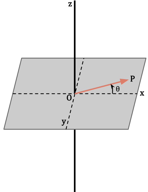
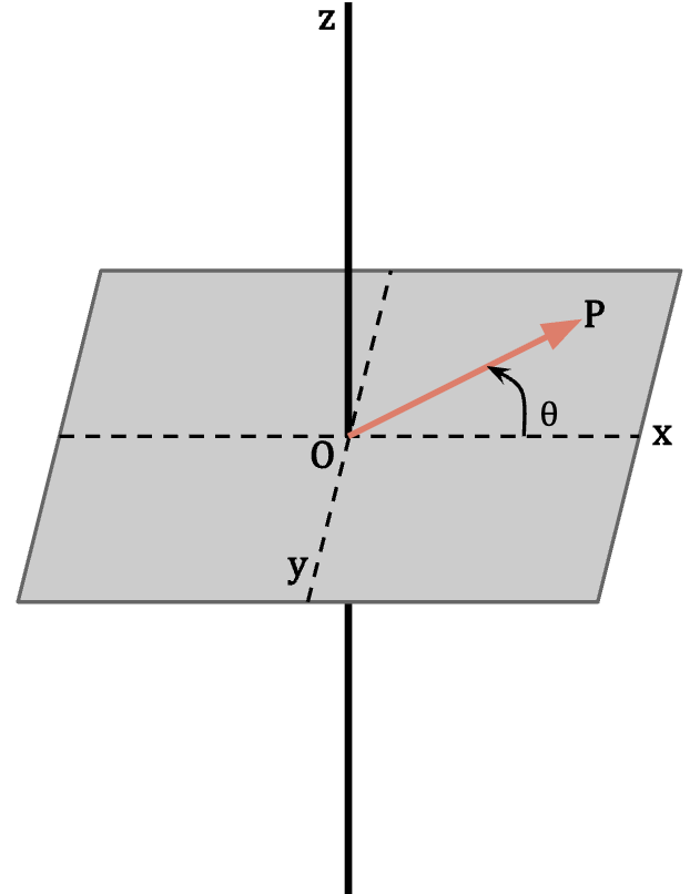
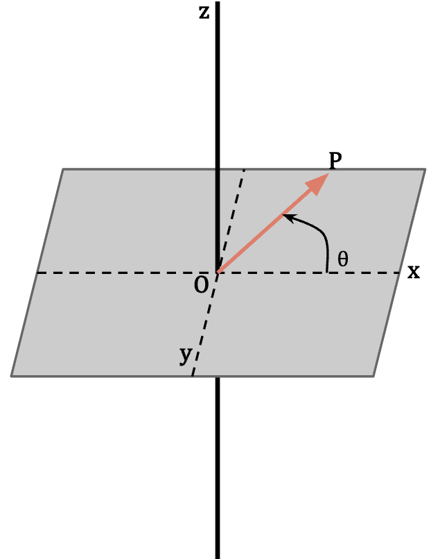
The graphic shows a rigid body, say a speedometer needle, that is rotating about a fixed axis. The body rotates in the xy-plane while it’s axis of rotation passes through the origin and is along the z-axis or in other words, is perpendicular to the plane of motion.

The motion of the body can be described using x- and y-coordinates of it’s location⁴ at each instant of time. However, since both x- and y-coordinates are changing with time, describing the rotation of a body in this manner is not very convenient.

Instead, notice in the graphic that there is a fixed line OP that is moving about the axis of rotation and the only variable quantity in that case is the angle $\theta$ that this line makes with the +x-axis⁵. $\theta$ can either be positive or negative depending on which direction of rotation you choose to be positive or negative⁶. Usually, positive direction of rotation is chosen to be counterclockwise. If that’s the case, for a body that is moving clockwise, $\theta$ is negative and for a body moving counterclockwise, $\theta$ is positive.

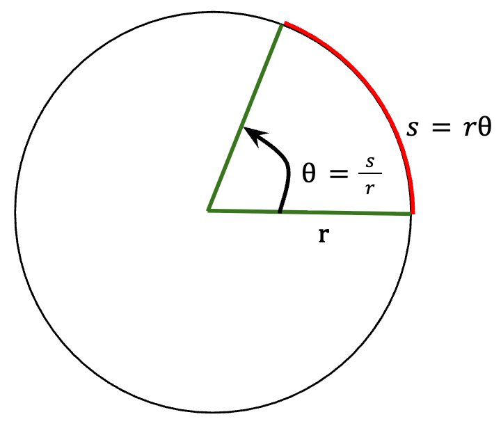
One way to measure the angle $\theta$ is in terms of radians. By definition, 1 radian (rad) is defined as the “angle subtended at the center of a circle by an arc with a length equal to the radius of the circle” (see figure 1).

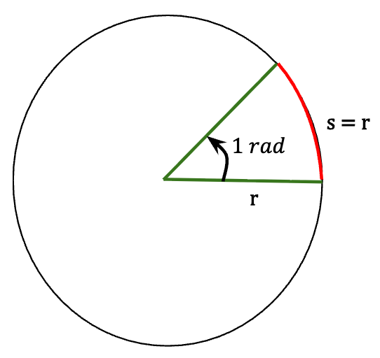
In other words, if you go along the curve of a circle and cover a distance s that equals the radius r of the circle, then you have turned by an angle that equals one radian.

This means that if you cover an arbitrary distance s along a circle of radius r, then the angle you turned in radians can be calculated as follows:

or

Note 1: $\theta$ is in radians in equations (1) and (2).

Note 2: The angle $\theta$ when measured in radians is a pure number with no units, since by definition, it is a ratio of two lengths. But the angle is often written as 1 rad or 2 rad in order to differentiate it from an angle given in degrees or revolutions.

Now, if you go around the full circle, you cover a distance $2\pi r$ (the circumference of a circle). Plugging this value into equation (1),

Since one revolution around the circle corresponds to an angle of 360°, we can deduce that;

or

Similarly, $\pi~rad = 180°$ and $\pi/2~rad = 90°$ and so on.

Angular Velocity

The rotational position of a rigid body at any instant can be given by it’s angular coordinate $\theta$. We can then describe the rotational motion of a body through the change in the angular coordinate $\theta$ with respect to time.

Consider a rigid body, say a speedometer needle (line OP in Figure 3), that is rotating about a fixed axis such that at time t = $t_1$, it’s angular coordinate is given by $\theta_1$. After some time $\Delta t$, the body’s angular coordinate is $\theta_2$ at time t = $t_2$. Note: the angular coordinate $\theta$ is measured from the positive x-axis.

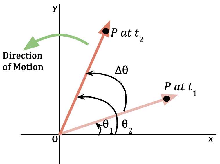
The average angular velocity ($\omega_{av-z}$) can then be defined as the rate of change of angular coordinate $\theta$ in the time interval $\Delta t$. In other words, it is the ratio of angular displacement $\Delta \theta$ over the time interval $\Delta t$;

Note: Even though we are just tracking the point P in figure 3, it is crucial to know that every point on the speedometer needle is moving with the same angular velocity $\Delta \theta/\Delta t$. In other words, each point has different $\theta_1$ and $\theta_2$ but $\Delta \theta$ over the time interval $\Delta t$ is the same for each point.

The subscript z in equation (6) depicts that the fixed axis around which the rigid body is rotating is in the z-direction.

Now, in the limit that $\Delta t$ approaches zero, the average angular velocity is equal to the instantaneous angular velocity ($\omega_z$) of the rigid body;

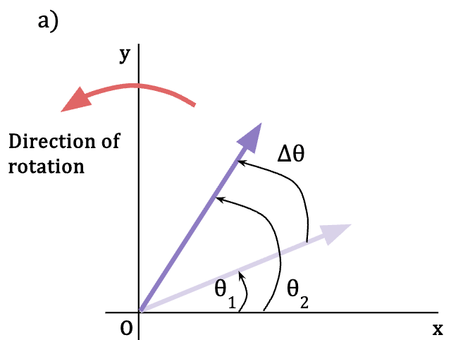
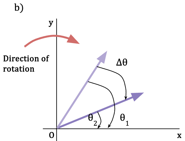
The angular velocity ($\omega_z$) of the rigid body can be positive, negative or zero. If we choose the positive direction of rotation to be counterclockwise, or in other words, we take $\theta$ to increase in the counterclockwise direction, then;

1. If the direction of rotation is counterclockwise, or $\theta$ is increasing ($\theta_2>\theta_1$), then the angular displacement $\Delta \theta$ is greater than zero and the angular velocity of the body is positive.
2. If the direction of rotation is clockwise or $\theta$ is decreasing ($\theta_2<\theta_1)$, then the angular displacement $\Delta \theta$ is less than zero and the angular velocity of the body is negative.
3. Lastly, if the body is not rotating, then the angular displacement $\Delta \theta$ is zero and so is the angular velocity.

However, angular speed ($\omega$) is the magnitude of angular velocity and thus, it is always a positive quantity.

If angular coordinate $\theta$ is measured in radians, then the unit of angular velocity is radian per second or rad/s.

Other commonly used units for angular velocity are: revolution per second or rev/s and revolutions per minute or rpm (rev/min).

1 rev/s = 2$\pi$ rad/s …..(8)

(because there are 2$\pi$ radians in one revolution).

1 rpm = $\frac{1}{60}$ rev/s = $\frac{2\pi}{60}$ rad/s…..(9)

Angular Velocity as a Vector

Similar to how a velocity vector $\vec{v}$ has a component in x-direction given by $v_x$, $\omega_z$ refers to the z-component of angular velocity, $\vec{\omega}$. The subscript z depicts that $\omega_z$ is the component of angular velocity vector that is rotating about the z-axis.

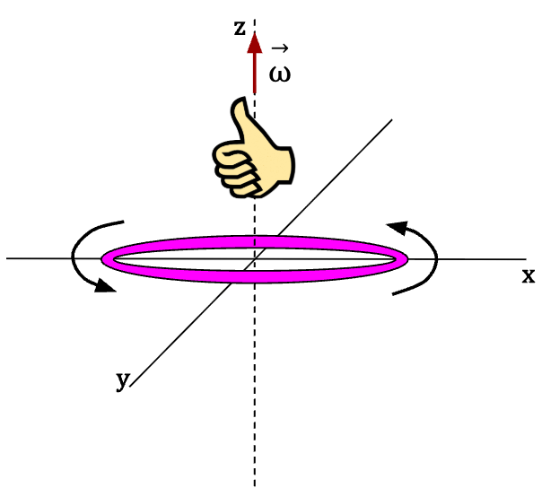
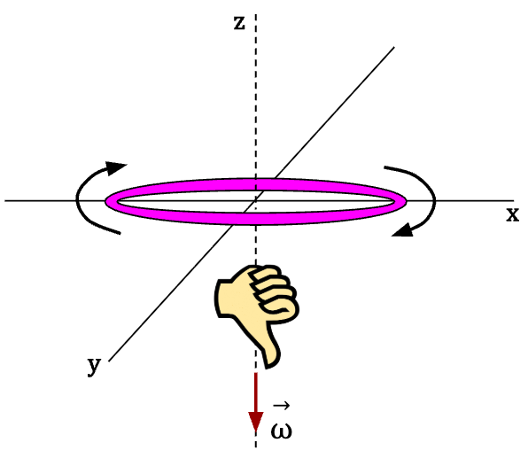
The direction of $\vec{\omega}$ is given by the right-hand rule. If you curl your fingers in the direction in which the rigid body is rotating, then the thumb points in the direction of angular velocity vector, $\vec{\omega}$⁷.

Angular Acceleration

When the angular velocity of a rigid body is changing, it is said to have angular acceleration. For example, friction provides angular acceleration to a tire when it stops it from rolling down a surface.

Consider a rigid body whose angular velocity is changing with time. Let it’s instantaneous angular velocity at time $t_1$ be $\omega_{z1}$ and at time $t_2$ be $\omega_{z2}$.

The average angular acceleration ($\alpha_{av-z}$) of the rigid body rotating about the z-axis over the time interval, $\Delta t = t_2-t_1$ is then given by;

In the limit that $\Delta t$ approaches zero, the average angular acceleration becomes equal to the instantaneous angular acceleration of the rigid body;

Angular acceleration is often measured in radian per second per second or rad/s².

Since $\omega_z = d\theta/dt$, we can rewrite equation (11) as;

In other words, the angular acceleration of a rigid body is equal to the second derivative of the angular coordinate with respect to time.

To distinguish angular quantities $\theta, \omega_z$ and $\alpha_z$ from straight line quantities x, $v_x$ and $a_x$; x is sometimes referred to as the linear displacement, $v_x$ as the linear velocity and $a_x$ as the linear acceleration.

If the angular acceleration $\alpha_z$ is positive, then the angular velocity of the rigid body, $\omega_z$ is increasing or $\omega_z$ is becoming more positive. On the other hand, if angular acceleration $\alpha_z$ is negative, then the angular velocity of the rigid body, $\omega_z$ is decreasing or $\omega_z$ is becoming more negative.

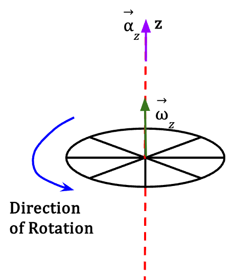
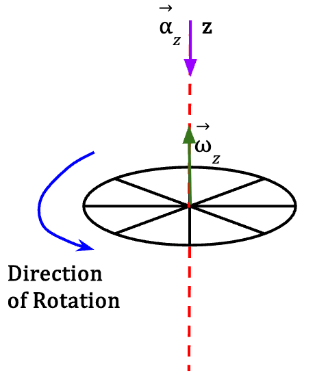
If the angular velocity and angular acceleration have the same sign, then the rigid body’s rotation is speeding up. However, if the angular velocity and angular acceleration have opposite signs, then the rigid body starts to slow down. For example, if a body is rotating in the counterclockwise direction, then the direction of angular velocity is along the positive z-direction. If the angular acceleration is also acting along the positive z-direction, then the rotation of the body will speed up. If instead, the angular acceleration acts along the negative z-direction, then the rotation of the body starts to slow down.

Angular Acceleration as a Vector

The angular acceleration vector, $\vec{\alpha}$ is defined as the rate of change of angular velocity vector $\vec{\omega}$ with respect to time. If the rotational axis is fixed⁸ (say the z-axis), then the angular acceleration and angular velocity lie along the same axis.

If angular acceleration acts along the same direction as angular velocity, then the rotation of the rigid body speeds up and if angular acceleration acts in a direction opposite to that of angular velocity, then the rotation of the rigid body slows down.

---

Rotation with Constant Angular Acceleration (Young et al., 2020)

When angular acceleration is constant, we can derive equations similar to kinematic equations derived for straight-line motion.

Consider a rigid body rotating about a fixed axis, say the z-axis that is acted upon by a force that produces a constant angular acceleration of $\alpha_z$. Let it’s initial angular velocity at time t = 0 be $\omega_{0z}$ and it’s final angular velocity and time t = t be $\omega_z$, then using equation (10), we can write;

or

The angular velocity of the rigid body during the time t changes by a factor $\alpha_zt$ and the final angular velocity ($\omega_z$) is equal to the initial angular velocity ($\omega_{0z}$) plus the change in the angular velocity ($\alpha_zt).$

Since the angular velocity of the rigid body is changing at a uniform rate because angular acceleration is constant, the average angular velocity is simply the average of the initial and final value of angular velocity between the time interval 0 and t;

If the angular coordinate of the rigid body at time t=0 is $\theta_0$ and at time t = t is $\theta$, then using equation (6) we can write;

Equating equations (15) and (16), we get;

Rearranging, we get;

Now, equation (14) can be substituted into equation (18) to get a relationship between $\theta$ and t that does not involve the angular velocity of the rigid body at time t ($\omega_z)$;

This means that the angular coordinate $\theta$ of the rigid body at time t is equal to the initial angular coordinate $\theta_0$, plus the change in angular coordinate if angular acceleration was zero and angular velocity was constant ($\omega_{0z}t$), plus the change in the angular coordinate due to the changing angular velocity caused by constant acceleration ($1/2\alpha_zt^2)$.

Now we can eliminate t in equation (21) to get a relationship between the angular velocity ($\omega_z$) and the angular coordinate ($\theta).$

From equation (14), we see that;

Plugging equation (22) into equation (21);

Cancelling the terms $\frac{\omega_{0z}\omega_z}{\alpha_z}$ & $-\frac{\omega_{0z}\omega_z}{\alpha_z}$ and multiplying both sides by the term $2\alpha_z$;

or

Comparing Angular and Straight Line Equations of Motion with Constant Acceleration

Straight-line Motion with Constant Linear Acceleration ($a_x$)	Fixed-Axis Angular Rotation with Constant Angular Acceleration ($\alpha_z$)
$v_x = v_{0x}+a_xt$	$\omega_z = \omega_{0z}+\alpha_zt$
$x = x_0 + v_{0x}t+\frac{1}{2}a_xt^2$	$\theta = \theta_0 + \omega_{0z}t+\frac{1}{2}\alpha_zt^2$
$v_x^2=v_{0x}^2+2a_x(x-x_0)$	$\omega_z^2=\omega_{0z}^2+2\alpha_z(\theta-\theta_0)$
$x-x_0 = \frac{1}{2}\big(v_{0x}+v_x\big)t$	$\theta-\theta_0 = \frac{1}{2}\big(\omega_{0z}+\omega_z\big)t$

where at time t = 0, the linear position is $x_0$, linear velocity is $v_{0x}$, the angular coordinate is $\theta_0$ and angular velocity is $\omega_{0z}$. Sometime later at time t=t, the linear position is $x$, linear velocity is $v_{x}$, the angular coordinate is $\theta$ and angular velocity is $\omega_z$.

---

Relating Linear and Angular Kinematics (Young et al., 2020)

It is important to develop a relationship between linear speed/acceleration and angular speed/acceleration of a rigid body that is rotating about a fixed axis because in order to evaluate the kinetic energy of a rotating rigid body, the linear speed $v$ is needed.

Linear Speed in Rigid-Body Rotation

Consider a rigid body that is rotating about a fixed axis. As the whole body rotates, each particle travels along a circular path in a plane that is perpendicular to the fixed axis.

Faster a body rotates, larger is the speed of the particle and hence, we can say that the linear speed of the particle is directly proportional to it’s angular velocity.

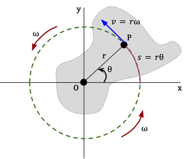
Now let’s look at a single particle P on this rotating rigid body. As the whole body rotates, the point P follows a circle of radius r (see figure 10). At any instant, the distance (s) that P moves is given by;

where $\theta$ is the angular displacement of point P measured in radians from the positive x-axis.

Taking derivative of equation (29) with respect to time;

Since radius r is constant for point P,

Taking absolute values on both sides of equation (31);

Now, $\abs{ds/dt}$ is equal to the instantaneous linear speed (v) of the particle because it is the absolute value of the rate of change of arc length (s) as the particle P rotates along the circular path. $\abs{d\theta/dt}$ is equal to the magnitude of instantaneous angular velocity ($\vec{\omega}$) and is referred to as the instantaneous angular speed ($\omega$) of the particle.

where v is the linear speed of a point on the rotating body, r is the distance of that point from the rotation axis and $\omega$ is the angular speed of the rigid body measured in rad/s.

We can see from equation (32) that farther is a point from the rotation axis (r), larger is it’s linear speed ($v$).

Note: Equation (32) is a relationship between magnitudes of linear velocity and angular velocity and thus, $v$ and $\omega$ are never negative. Additionally, the equation does not give any information regarding the direction of linear or angular velocity. It only tells you how fast a point is travelling ($v$) as the rigid body rotates or how fast the rigid body is rotating ($\omega)$. The direction of linear velocity is always tangent to the circular path that the point is moving along. The direction of angular velocity is either positive or negative as given by the right-hand rule.

Linear Acceleration in Rigid-Body Rotation

The acceleration $\vec{a}$ of a rotating body can be broken into two components: tangential acceleration ($a_{tan}$) and centripetal acceleration ($a_{rad}$). The tangential component, as the name suggests, lies on the tangent to the circle along which a particle on the rotating body is moving. The centripetal component acts along a direction that is perpendicular to the moving particle and points towards the centre of the circular path.

The tangential component of acceleration changes the magnitude of particle’s velocity depending on whether the acceleration acts parallel or antiparallel to the velocity vector. It’s magnitude is equal to the derivative of the linear speed of the particle;

Since r, the distance of the particle from the rotation axis, is constant;

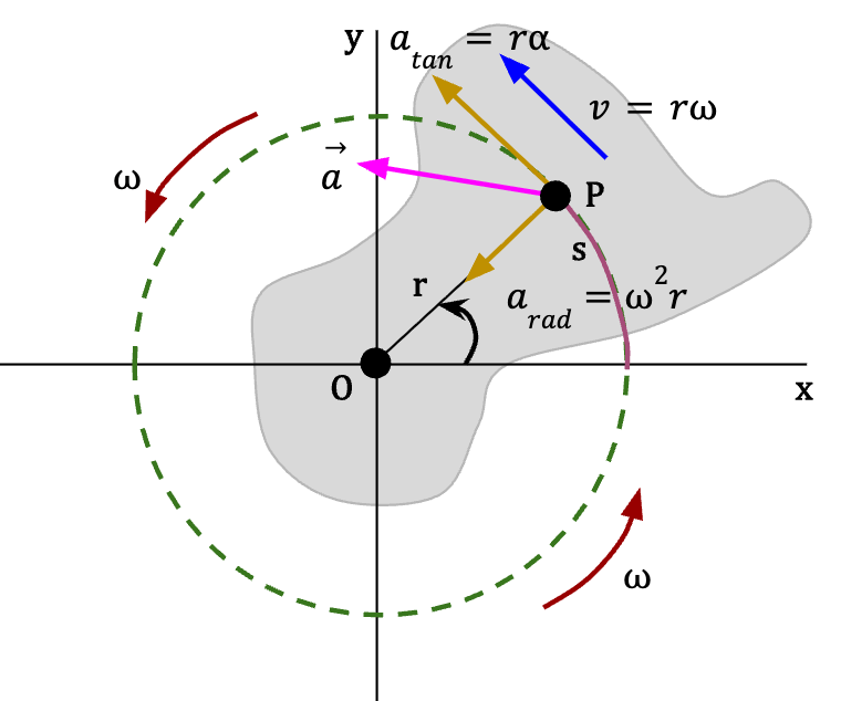
It is important to understand the distinction between $\alpha = d\omega/dt$ and $\alpha_z = d\omega_z/dt$. $\alpha$ is the rate of change of angular speed whereas $\alpha_z$ is the rate of change of angular velocity.

Thus, for fixed axis rotation, if $\omega_z$ is positive, then;

However, if $\omega_z$ is negative, then;

For example, consider a body rotating about a fixed axis that is along the z-direction. If, $\omega_z$ is positive, then the body is rotating counterclockwise and according to the right hand rule the direction of $\omega_z$ is along the positive z-direction. If the body is speeding up, then $\alpha$ is positive because during the infinitesimal time interval dt, the final angular speed ($\omega$) is larger than initial $\omega$. Additionally, $\alpha_z$ is positive because the body’s angular velocity ($\omega_z$) is becoming more positive. However, if the body is slowing down, then the angular speed is decreasing with time and $\alpha$ is negative. $\alpha_z$ is also negative because $\omega_z$ is becoming less positive with time.

If $\omega_z$ is negative or if body is rotating clockwise and the body is speeding up, then $\alpha$ is positive because angular speed $\omega$ is increasing with time. However, $\alpha_z$ is negative because $\omega_z$ is becoming more negative with time. On the other hand, if the body is slowing down, then $\alpha$ is negative because angular speed $\omega$ is decreasing with time but $\alpha_z$ is positive because the angular velocity $\omega_z$ is becoming less negative with time.

The radial component of acceleration ($a_{rad}$) is responsible for changing the direction of the rotating point on a rigid body and is equal to $v^2/r$.

Using equation (32), we can say;

where r is the distance of the point from rotation axis and $\omega$ is the angular velocity of the point.

This relationship holds true at each instant of time even when linear speed $v$ and angular speed $\omega$ are not constant.

The radial component of acceleration is always perpendicular to the direction of motion and points towards the rotational axis at all times.

Note 1: The requirement for using equations (32), (34) and (37) is that $\omega$ is measured in rad/unit of time and $\alpha$ is measured in rad/unit of time squared. The unit of time can be s, min, ms etc.

Note 2: Equations (29), (32) and (34) are also applicable to any particle that has the same tangential velocity as the point on the rigid body that is rotating around a fixed axis. For example, when a bicycle chain turns with a rotating sprocket without slipping or deforming, it has the same velocity and tangential acceleration as the sprocket itself.

The same can be said about a belt and pulley system, given that the belt turns without slipping or stretching.

However, equation (37) is only applicable to points that are connected to the rotating rigid body. For example, in the case of sprocket and bicycle chain system, the radial acceleration given by equation (37) holds true only for parts of the chain that are connected to the rotating sprocket.

---

Energy in Rotational Motion (Young et al., 2020)

When a rigid body is rotating about a fixed axis, at each instant, the particles on the rigid body have tangential velocity and therefore, also have kinetic energy.

Consider a rotating rigid body that is made up of n particles with masses $m_1,~m_2,~m_3,……….,~m_n$ that are located at a distance $r_1,~r_2,~r_3,………,~r_n$ respectively from the rotation axis (it is not necessary for all the particles to lie in the same plane).

The kinetic energy of the $i$th particle is given as;

where $m_i$ is the mass of the $i$th particle, $v_i$ is the tangential speed of the $i$th particle and $i = 1, 2, 3,……..,n$.

From equation (32), we have;

where $r_i$ is the perpendicular distance of the $i$th particle from the rotation axis and $\omega$ is the angular speed of the rigid body measured in rad/s.

Substituting equation (39) into equation (38), we get;

The total kinetic energy of the rigid body (K) rotating about a fixed axis is the sum of all the kinetic energies of each particle;

where

Taking common factor $1/2\omega^2$ out of the expression in equation (42);

We can now define a quantity called Moment of Inertia ($I$) for a given rotation axis and it equals;

The word moment does not mean a moment in time, rather it describes that the quantity $I$ depends on how a body’s mass is distributed in space. When dealing with objects with a continuous distribution of matter, for example, a solid sphere, the sum in equation (44) needs to be changed to an integral and calculus is needed to evaluate the moment of inertia of the rigid body.

For a rigid body, the quantities $m_i$ and $r_i$ are constant for each particle and thus, moment of inertia $I$ does not depend on how a body rotates in space and time.

The SI unit of $I$ is $kg~ \dot{} ~m^2$.

We can now rewrite equation (41) as;

where $\omega$ is measured in rad/s.

From equation (44) and (45) we see that, greater are the distances of particles from the rotation axis, larger is the moment of inertia. Larger is the moment of inertia of a rigid body rotating about an axis with angular speed $\omega$, larger is it’s kinetic energy.

Kinetic energy of a rigid body can be defined as the amount of work needed to accelerate it from rest. This means that larger is the moment of inertia of a rigid body, larger is the kinetic energy needed to initiate rotation in a body at rest. Conversely, larger is the moment of inertia of a rigid body, larger is the kinetic energy needed to stop it from rotating. This is why moment of inertia ($I$) is also referred to as the rotational inertia.

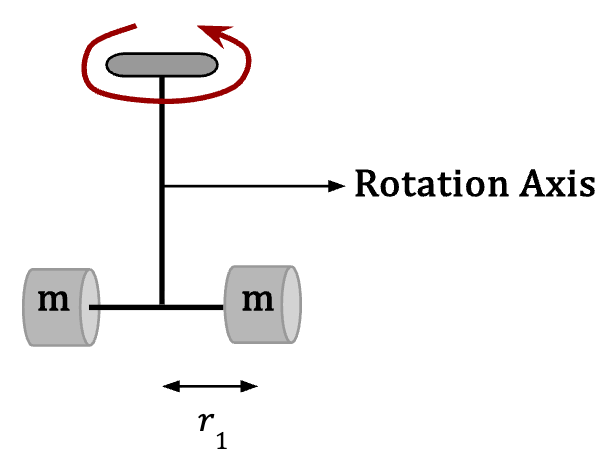
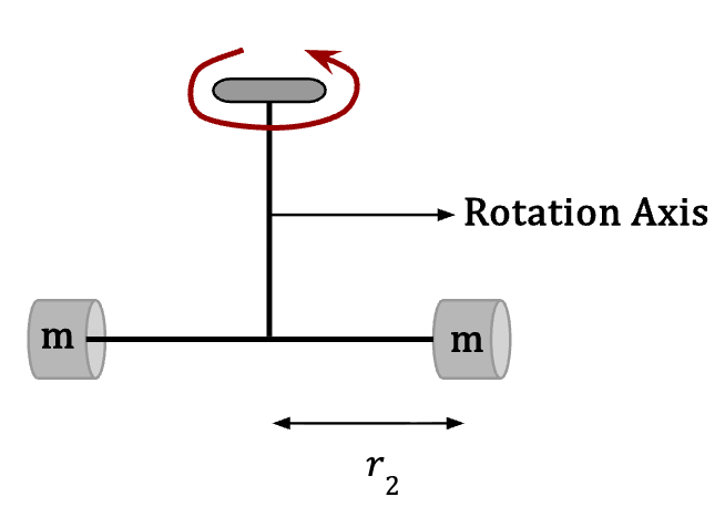
Since the distance $r_2$ in figure 14 is larger than $r_1$ in figure 13, the moment of inertia of apparatus in figure 14 is greater and therefore, larger amount of kinetic energy is required to get it to start rotating.

Note: Moment of inertia of a rigid body depends on which axis of rotation you choose.

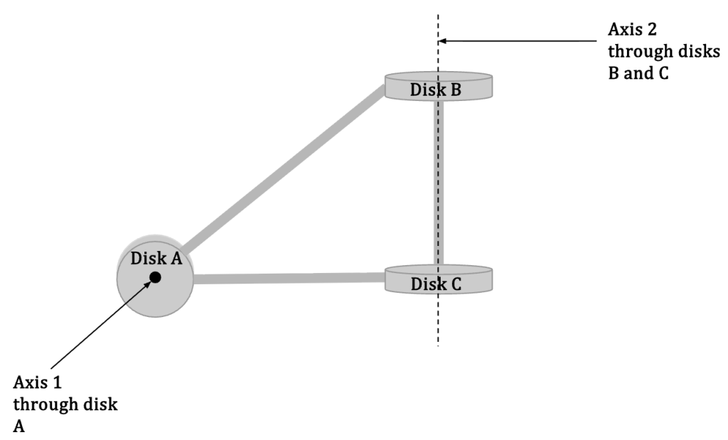
In figure 15, axis 1 is located through the disk A and is perpendicular to the plane of the diagram (the axis is coming out of the screen) and axis 2 is located through disks B and C with orientation as shown in the diagram. The moment of inertia through axis 1 and axis 2 will most likely not be the same. Depending on which moment of inertia is smaller, easier it will be to rotate the machine part around that axis.

See the table below for moments of inertia of several bodies with uniform distribution of matter (density is the same throughout the object);

Type of object with the choice of axis	Diagram with dimensions as shown	Moment of Inertia
Slender Rod of mass M, with axis through the center		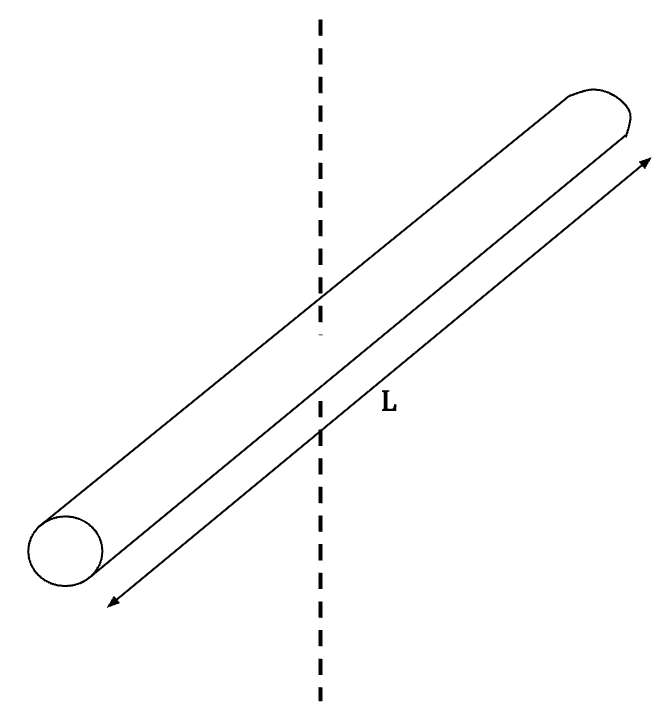$I = \frac{1}{12}ML^2$
Slender Rod of mass M, with axis through one end		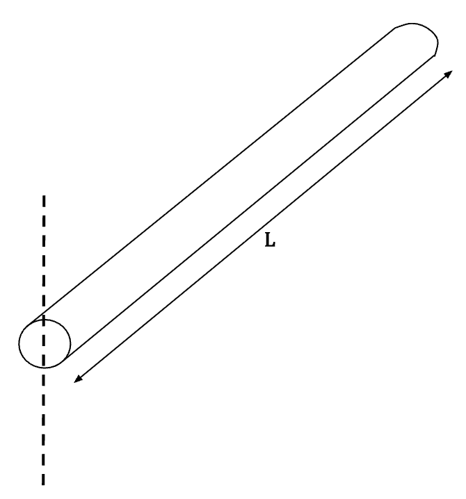$I = \frac{1}{3}ML^2$
Rectangular Plate of mass M, with axis through the center		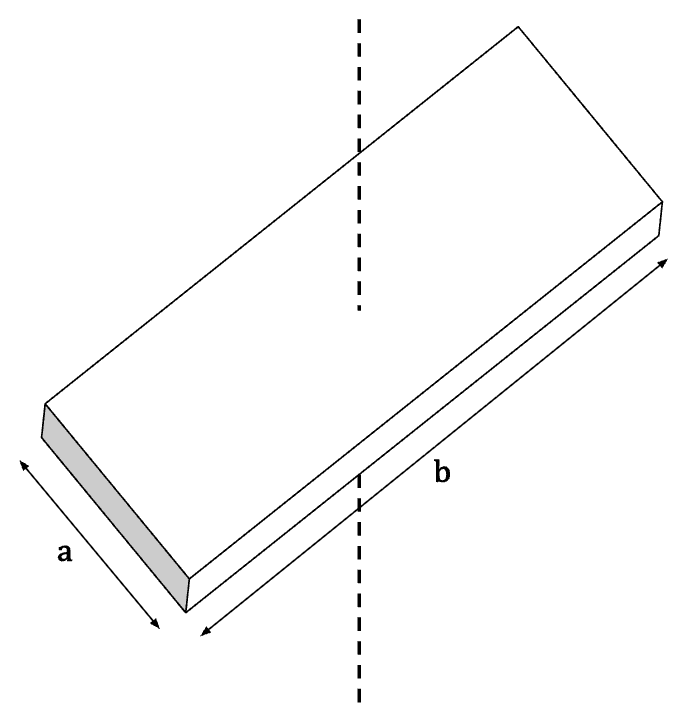$I = \frac{1}{12}M(a^2+b^2)$
Thin Rectangular Plate of mass M, with axis along the edge		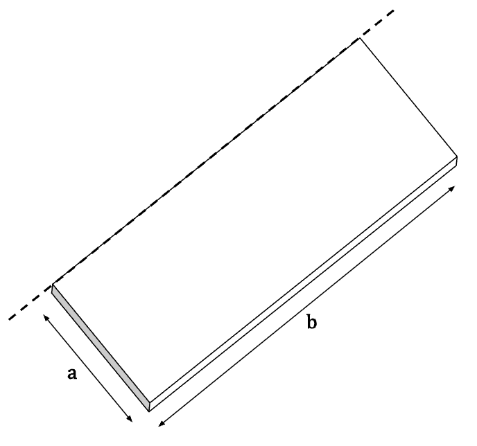$I = \frac{1}{3}Ma^2$
Hollow Cylinder of mass M, with axis through the middle		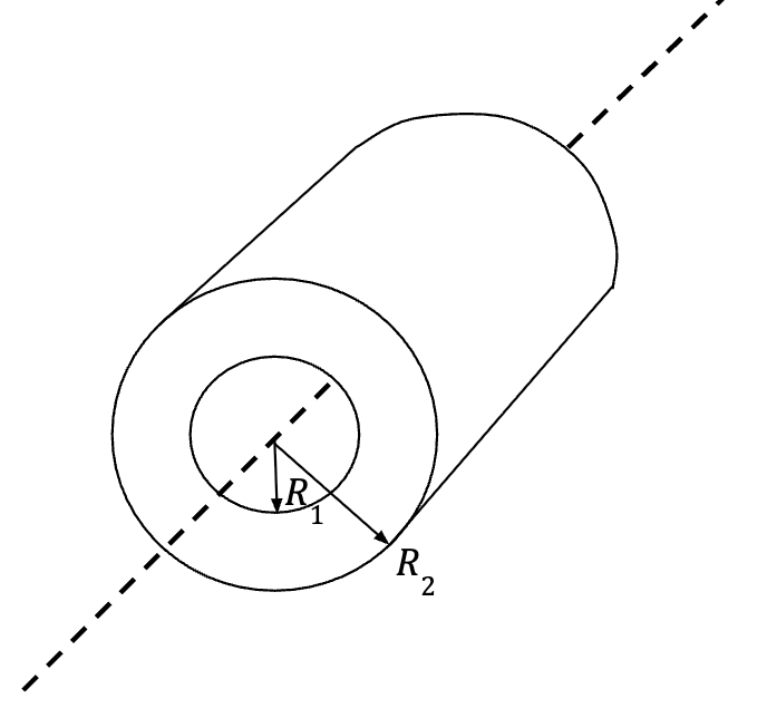$I = \frac{1}{2}M(R_1^2+R_2^2)$
Solid Cylinder of mass M, with axis through the middle		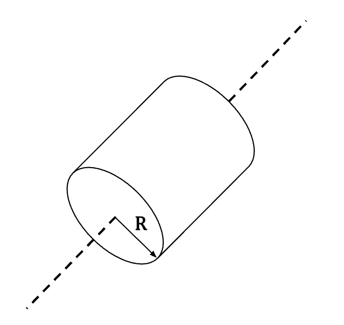$I = \frac{1}{2}MR^2$
Thin-Walled Hollow Cylinder of mass M, with axis through the middle		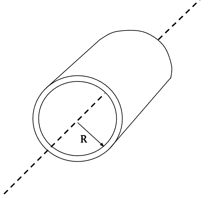$MR^2$
Solid Sphere of mass M, with axis through the middle		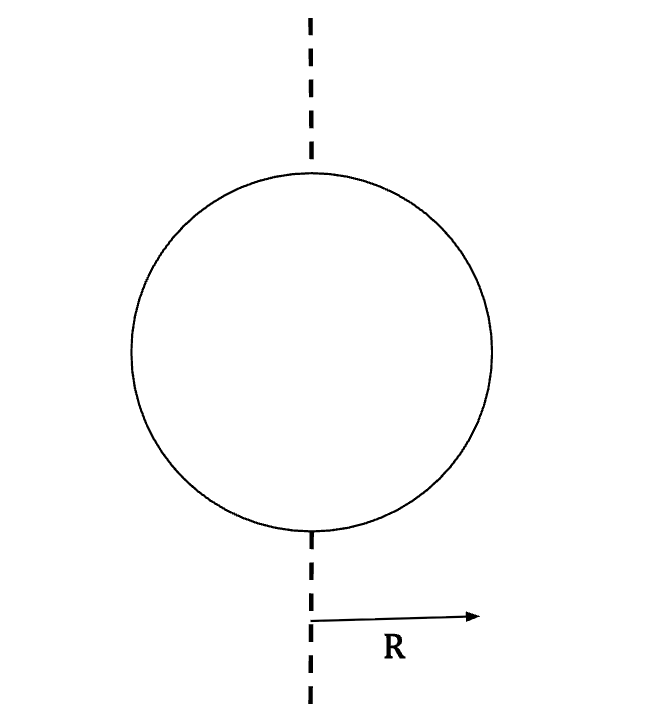$\frac{2}{5}MR^2$
Thin-Walled Hollow Sphere of mass M, with axis through the middle		$\frac{2}{3}MR^2$

Common Misunderstanding

In order to calculate moment of inertia, it is a common mistake to assume that all of a body’s mass is concentrated at the center of the rigid body and then multiply it with the square of the distance of the center of mass from the rotation axis. However, this would yield an incorrect answer. For instance, for a slender rod of length L with rotational axis through it’s one end (as shown in the second row of the table above), the center of mass is a distance L/2 away from the rotation axis. This would give $I = M(L/2)^2 = ML^2/4$ which as you can see would be an incorrect answer.

Gravitational Potential Energy for an Extended Body

For a mass m attached to a pulley with a cable, the gravitational potential energy of the cable can be ignored if the cable has negligible mass. However, for a cable of substantial mass, it’s gravitational potential energy need to be taken into consideration when using energy methods to solve problems.

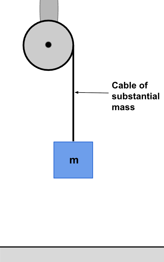
If the extended object, like the cable in figure 16, has same value of acceleration due to gravity (g) at all points, then we can assume that all of the extended body’s mass (M) is concentrated at the center of mass. If we take upward direction to be positive and the y-coordinate of the center of mass as $y_{cm}$, then the gravitational potential energy is given as;

Equation (46) is applicable to any extended body, regardless of whether it is rigid or not.

Proof of Equation (46):

Suppose the cable in figure (16) is made up of n number of particles with mass $m_1, m_2, m_3,……., m_n$ with y coordinate given as $y_1, y_2, y_3,…….,y_n$ respectively.

The total potential energy of the entire cable is the algebraic sum of potential energies of each of these particles;

From the definition of center of mass, we see that;

Since $m_1+ m_2+ m_3+……….+m_n = M$, equation (48) reduces to;

---

Parallel-Axis Theorem (Young et al., 2020)

A rigid body has infinite number of moment of inertia depending on infinite axes it can rotate about.

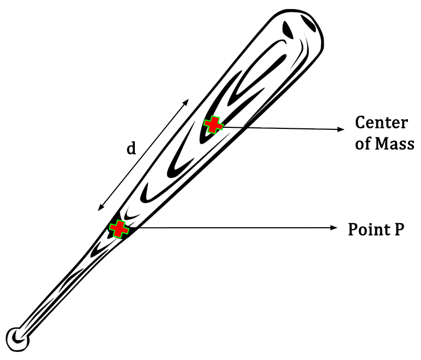
Parallel-axis theorem gives a relationship between the moment of inertia of the body rotating about an axis through it’s center of mass and moment of inertia about any other axis that is parallel to the axis going through the center of mass;

where $I_P$ is the moment of inertia of the rigid body rotating about an axis going through a point P (figure 17), $I_{cm}$ is the moment of inertia about an axis through the body’s center of mass and parallel to the axis going through point P, $M$ is the mass of the rigid body and $d$ is the distance between the two parallel axes.

Proof of Parallel-Axis Theorem:

Consider a rigid body of mass M with an axis through it’s center of mass (Axis 1) and a second axis through a point P (Axis 2). Axis 1 and Axis 2 are parallel to each other and are along the z-direction (see figure 18).

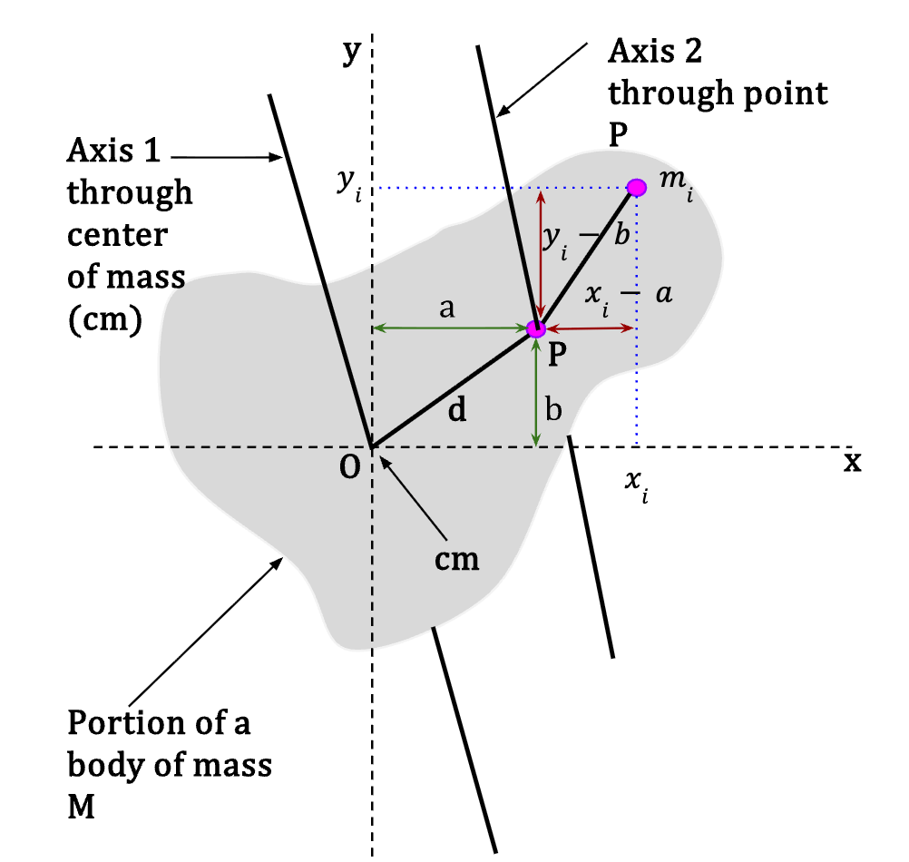
We then take a thin slice of this body that lies in the xy-plane and is perpendicular to the z-direction along which the two axes lie. Taking origin to be at the location of the center of mass (cm) of the body, we get the following coordinates $\{x, y, z\}$ for center of mass and point P;

Since Axis 1 passes through point O and Axis 2 passes through the point P, the distance (d) between the two axes has the following relationship;

Let $m_i$ be a small mass element at location $\{x_i,y_i,z_i\}$. The distance ($r_{i0}$) of this mass element from Axis 1 is equal to;

The moment of inertia of the slice about an axis through the center of mass is then give as;

The distance ($r_{iP}$) of the mass element $m_i$ from Axis 2 is equal to;

Note: The expressions in equation (55) and (57) do not include the coordinate $z_i$ because the axes 1 and 2 are perpendicular to the z-axis.

The moment of inertia of the slice about an axis that goes through the point P is given as;

Since the expressions in equation (56) and (58) do not include the coordinate $z_i$, the sums can be expanded to include all the particles in every thin slice along the z -axis such that the expressions then describe the moment of inertia of the entire body rotating about axis 1 and 2 respectively.

Expanding the squared terms in equation (58);

Regrouping equation (59), we get;

By definition of center of mass;

Since we took center of mass of the body to be at the origin, using equation (52);

This implies that;

Thus, the terms $2a\sum_im_ix_i$ and $2b\sum_i m_i y_i$ equal zero in equation (60).

Using equation (56), we see that the first term in equation (60) equals the moment of inertia of the rigid body rotating about an axis that goes through it’s center of mass, using equation (54) we see that $a^2+b^2$ in equation (60) equals $d^2$ and $\sum_im_i$ in equation (60) simply equals the total mass (M) of the rigid body. Plugging these into equation (60), we see that;

which is in agreement with equation (51).

We can deduce from equation (65) that the moment of inertia about an axis through some point P on the rigid body is larger than the moment of inertia about an axis through it’s center of mass. Thus, it is easiest for a body to start rotating about an axis through it’s center of mass.

---

Moment-of-Inertia Calculations (Young et al., 2020)

For rigid bodies with a continuous distribution of matter, such as solids, the sum in equation (44) needs to be switched to an integral.

Consider a rigid body that you divide into small elements of mass $dm$. The rigid body needs to be divided in such a manner that all of the particles in a single element are approximately at the same perpendicular distance ($r$) from the rotation axis. The moment of inertia can then be calculated as;

To evaluate the integral in equation (66), the elements $r$ and $dm$ need to be represented using the same integration variable.

For one-dimensional rigid bodies, for example a slender rod, the distance $r$ from the rotation axis can be represented using the variable $x$ and a relationship between $dm$ and a small increment of length $dx$ can be established. This allows us to represent the integral in equation (66) in terms of a single variable $x$.

However, when you are given a three-dimensional rigid body, the best course of action is to use the relationship $\rho = dm/dV$, where $\rho$ is the density of the rigid body and $dV$ is a small element of volume. Using this, equation (66) can be written as;

Equation (67) shows that the moment of inertia of a rigid body depends on “how it’s density varies within its volume”.

If the density $\rho$ is uniform or constant, it can be brought out of the integral and we get;

where $dV$ needs to be represented “in terms of the differentials of the integration variables”, for example $dV = dx~dy~dz$.

Note: For the integral in equations (67) and (68) to work, the volume element $dV$ must be chosen such that each and every point in the rigid body is approximately at the same distance ($r$) from the rotation axis.

Fun Fact

Geophysicists can measure the Earth’s moment of inertia by using the slight variations in the orbits of satellites revolving around Earth. From the calculated moment of inertia, it has been determined that Earth is much denser at the core when compared to the layers closer to the surface.

---

1. Young, H.D. et al. (2020) Sears and Zemansky’s university physics: With modern physics. 15th edn. Boston: Pearson. ↩︎
2. In reality, when objects are rotating, the forces can cause deformation whereby objects can get stretched or squeezed or twisted. A rigid body is an idealized object that retains its shape and structure while rotating. ↩︎
3. An axis that is stationary with respect to some inertial frame of reference such that it doesn’t move or change direction with respect to that frame is referred to as a fixed axis. ↩︎
4. Since the body in question is not a point particle, it’s motion can be described using a single point on this body (for instance, the very edge of the speedometer needle) and tracking it’s location as it changes with respect to time. ↩︎
5. x- and y- coordinates are referred to as Cartesian coordinates whereas $\theta$ is called an angular coordinate. ↩︎
6. This is similar to motion of a particle in the cartesian coordinate system whereby, you need to choose which direction is positive x and y. For example, for a projectile moving under the influence of gravity, you may choose positive x to be towards the right and positive y to be downwards. ↩︎
7. Note: Angular velocity and it’s corresponding rotational axis is common to the whole body, not just some part of the rigid body in question. ↩︎
8. Rotational axis does not have to be fixed, it can change direction as the body rotates with time. ↩︎