

List of Sources:
- Young et al., 20161
- Photo by cottonbro studio on Pexels.com
- Graphs generated using Desmos.com
Table of Contents:
- Displacement, Time and Average Velocity (Young et al., 2016)
- Instantaneous Velocity (Young et al., 2016)
- Average and Instantaneous Acceleration (Young et al., 2016)
- Motion with Constant Acceleration (Young et al., 2016)
- Free Falling Bodies (Young et al., 2016)
- Motion when Acceleration is not Constant (Young et al., 2016)
- Common Errors in Understanding (Young et al., 2016)
Displacement, Time and Average Velocity (Young et al., 2016)
For the purposes of understanding motion, macroscopic objects are often treated as particles.
Displacement
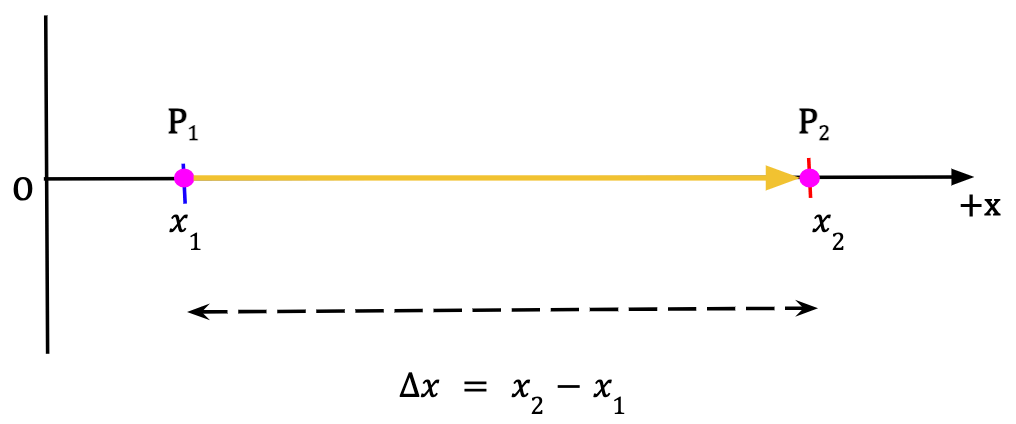
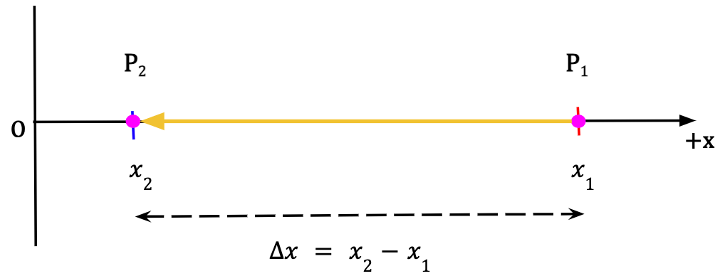
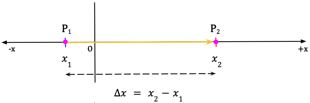
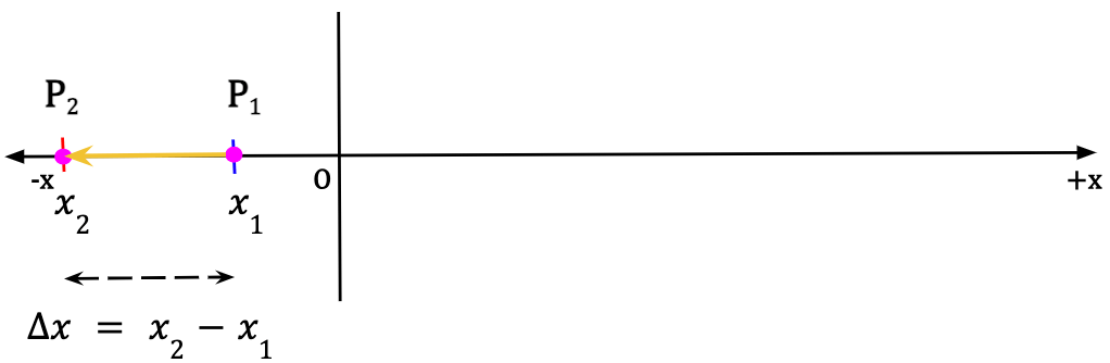
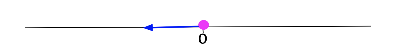
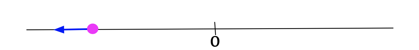
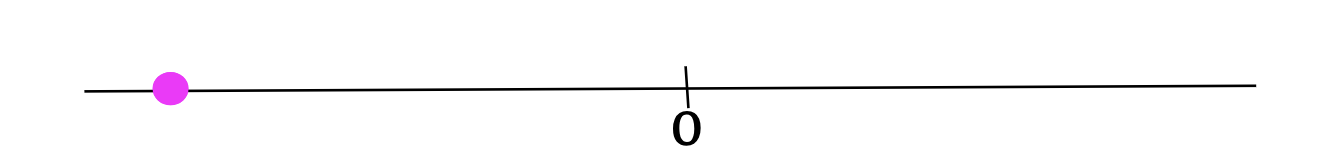
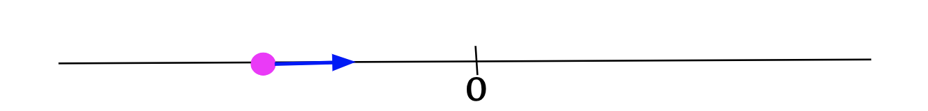
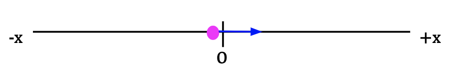
Consider a particle in 1D located at point P1 along the x-axis at time t1. After some time, the particle is found to be at point P2 at time t2. The component of the displacement vector along the x-direction is given by the change in the particle’s position which is equal to the difference between final position, given by the x-coordinate x2, and the initial position, given by the x-coordinate x1.
In other words, component of displacement along the x-axis is given by;
Δx2 = x2 – x1……(1)
The change in position occurs only along the x-axis which means that the y and z components of the displacement vector will be equal to zero, i.e., Δy = Δz = 0.
The direction of the displacement vector is towards the positive x-axis as depicted by the vector in Figure 1. In other words, if the particle’s initial position is positive and it starts to become more positive, we can conclude that it is moving towards the positive x-direction.
Time
The time interval is defined as the change in time as the particle displaces from point P1 to P2. This can be written as,
Δt = t2 – t1……(2)
Average Velocity
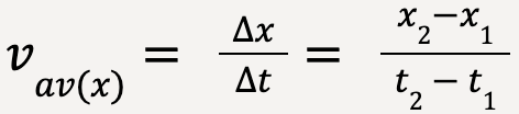
The average x-velocity (or component of average velocity along the x-direction) is then given as the component of the displacement vector along the x-axis divided by the time interval;
 …..(3)
If x is given in meters (m) and t in seconds (s), Δx/Δt has units of m/s which correctly correspond to the units of velocity. The direction of average x-velocity of the particle in Figure 1 is positive3 since the displacement vector is positive4.
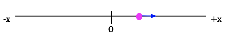
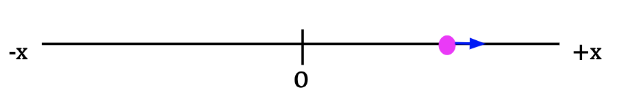
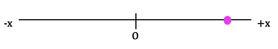
Scenario 1 is illustrated in Figure 1. The other three scenarios are shown below:
Scenario 2:
Scenario 3:
Scenario 4:
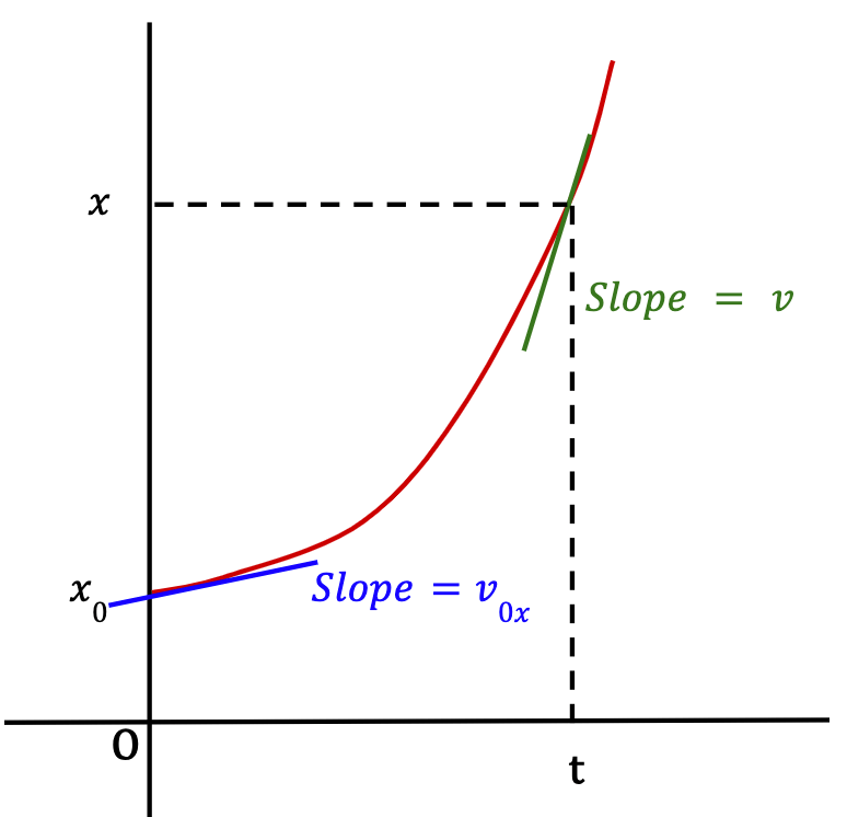
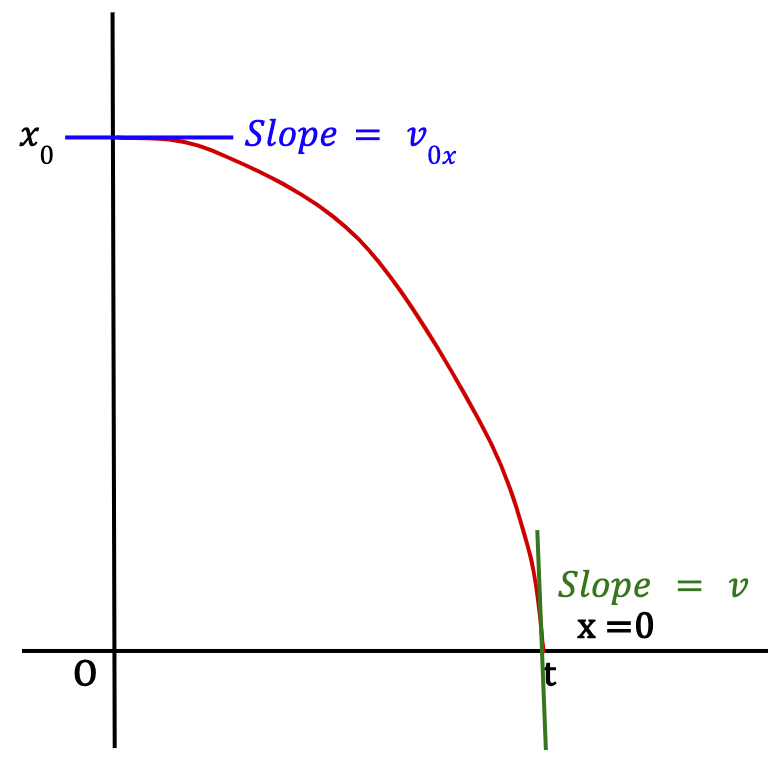
Graphical Representation
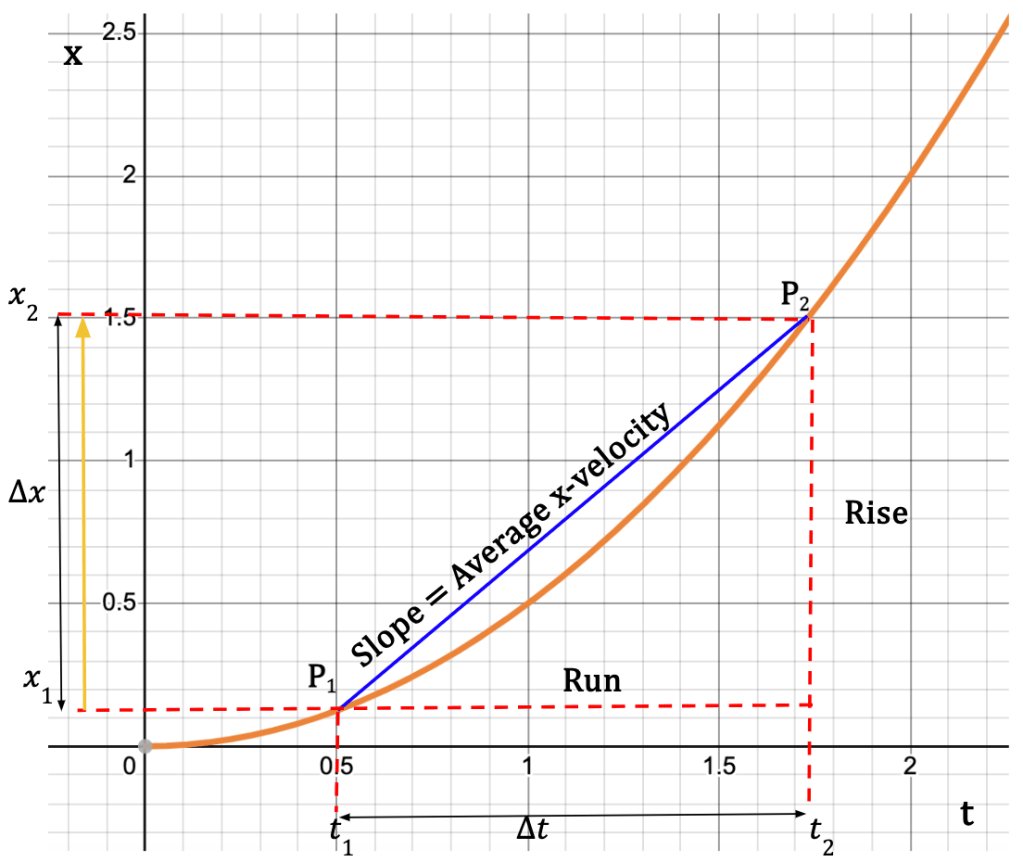
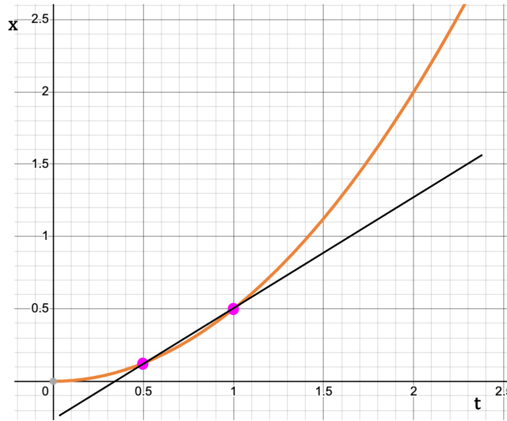
Figure 5: Graph of position (x) vs. time (t) is called an x-t graph. The orange curve represents the change in particle’s position with respect to time5. The difference between points P1 and P2 on the y-axis equals the displacement, and the difference on the x-axis is equal to the time interval. The slope of the line that connects points P1 and P2 gives the average x-velocity of the particle, such that, slope = rise/run = Δx/Δt.
Just like displacement is independent of the path taken by the particle, average velocity is independent of the particle’s velocity at any instant between points P1 and P2.
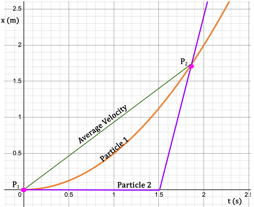
Figure 6: Particle 1 and Particle 2 start at the same point P1 (t1 = 0s). Between times t1 and t2, Particle 1 moves steadily while particle 2 remains at rest until t = 1.5s and then moves rapidly such that at t2 ≈ 1.85s both particles are at point P2. Since Δx and Δt are same for both the particles between points P1 and P2, so is the average x-velocity for Δt ≈ 1.85s – 0s ≈ 1.85s .
Instantaneous Velocity (Young et al., 2016)
If in Figure 1, we start moving P2 closer to P1 such that Δx and Δt become infinitesimally small, the instantaneous velocity is given by the average x-velocity in the limit that Δt approaches zero, which is also called the derivative of x with respect to t.
 …….(4)
The derivative of x with respect to t is described as the instantaneous rate of change in particle’s position. Similar to average x-velocity, the direction of instantaneous velocity is the same as the direction of the displacement vector6 (See Error #1).
Note: Instantaneous velocity (not average velocity) is what is meant when the word ‘velocity’ is used by itself.
Graphical Representation
The instantaneous velocity of a particle, vx can be determined from the x-t graph.
As the second point starts to approach the first one on x-t curve, the slope of the line between the two points approaches the slope of the tangent to the curve drawn at the first point (see below).
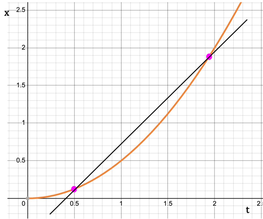
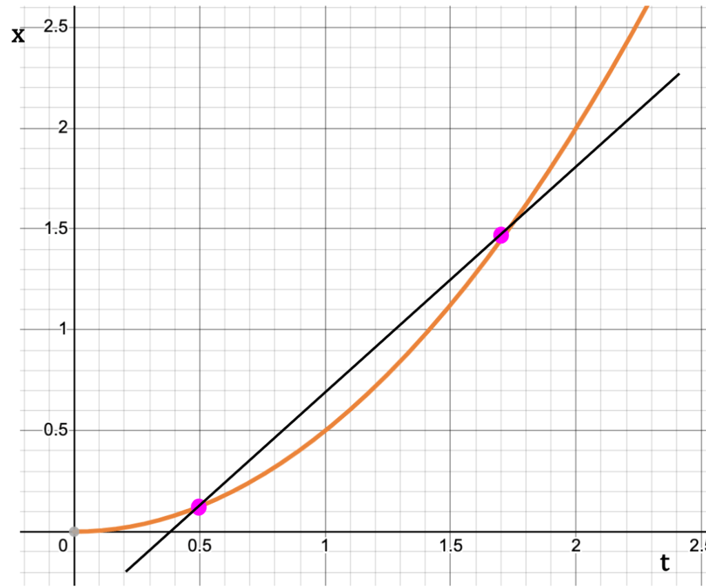

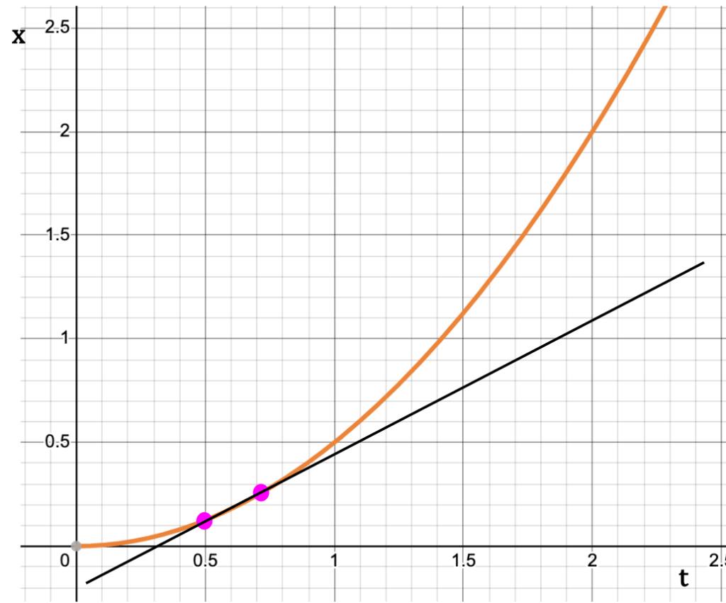

Thus, the instantaneous x-velocity at a point, say P1 on the x-t graph is equal to the slope of the tangent to the curve drawn at that point.

The Slope
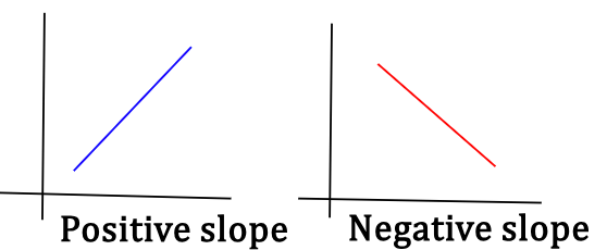
The direction of the slope, whether it is positive or negative gives information about the direction of instantaneous velocity. If the slope is inclined upwards on the right (positive slope), velocity is in the positive x-direction. Conversely, if the slope is inclined downwards on the right (negative slope), velocity is in the negative x-direction.
The steepness of the slope sheds light on the magnitude of the instantaneous velocity. Steeper the slope, faster is the particle moving.
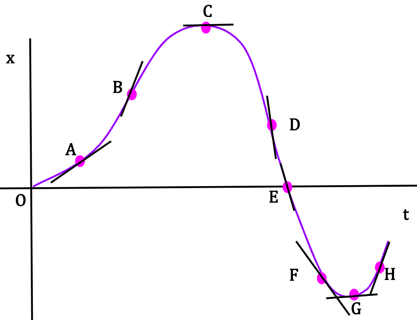
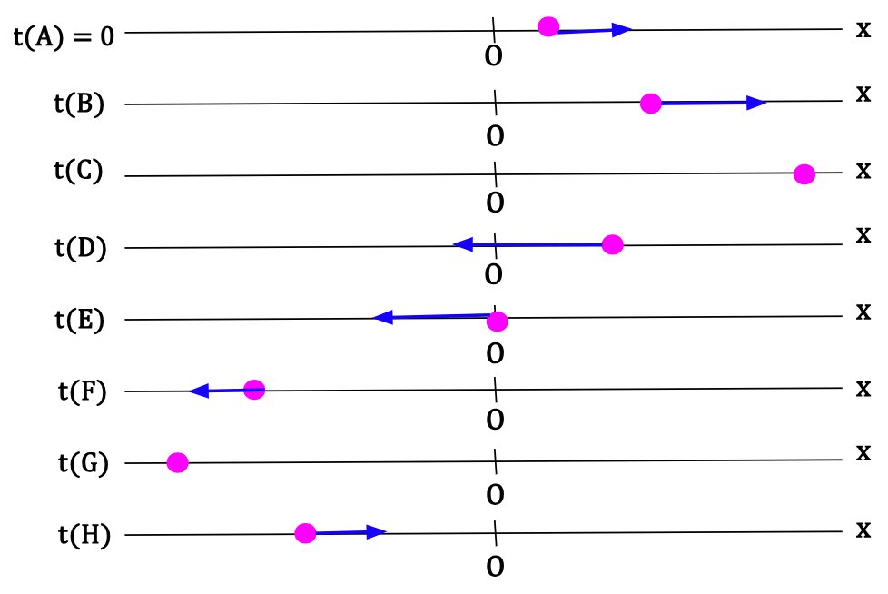
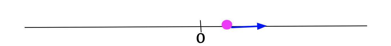
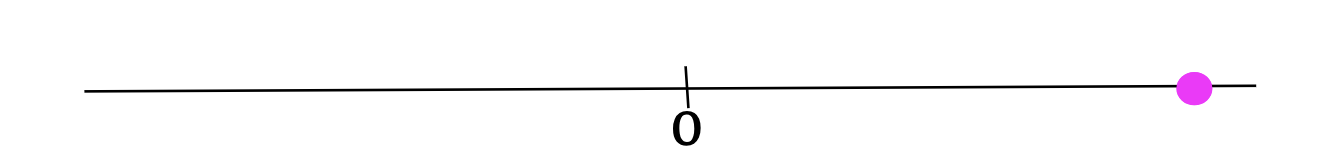
| Position | Position along x-axis7 | Slope | Particle’s position getting... | vx (direction) | vx (comparative magnitude) |
| A | On positive x-axis | Positive | …more positive | Positive x-direction | Not too steep, particle is picking up speed |
| B | On positive x-axis | Positive | …more positive | Positive x-direction | Much steeper, particle traveling much faster than position A |
| C | On positive x-axis | Zero | Momentarily at rest | N/A | Particle reached a maximum on the curve* and momentarily vx = 0 |
| D | On positive x-axis | Negative | …less positive | Negative x-direction | Very steep, particle moving very fast |
| E | At x=0 | Negative | Switching from positive to negative | Negative x-direction | Quite steep, but particle not as fast as at position D |
| F | On negative x-axis | Negative | …more negative | Negative x-direction | Steepness significantly dropped compared to position E, particle is slowing down |
| G | On negative x-axis | Zero | Momentarily at rest | N/A | Particle reached a minimum on the curve* and momentarily vx = 0 |
| H | On negative x-axis | Positive | …less negative | Positive x-direction | Getting steep again as particle picks up speed |
*Maximum and minimum on a curve simply describe the highest and lowest points on the curve indicative of the function flipping its direction. They do not correspond to maximum or minimum velocity of the particle. Velocity of the particle at both points is zero. At position C, the particle is farthest from origin along the positive x-axis and at position G, it is farthest from origin along the negative x- axis.
Motion Diagram
A Motion Diagram is used to show the position of a particle at certain instants of time with arrows that indicate the direction of the instantaneous velocity at that instant. The size of the arrow is equivalent to the magnitude of the instantaneous velocity. Larger is the size of the arrow, greater is the speed.
When the position of the particle at each instant in the motion diagram is stacked up sequentially, it creates a movie showing the movement of the particle along the x-axis (see below).

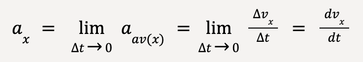
Average and Instantaneous Acceleration (Young et al., 2016)
In general, acceleration is a vector quantity that describes the rate of change of the velocity vector.
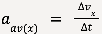
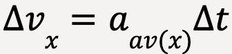
Average Acceleration
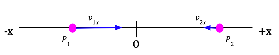
Consider a particle in 1D moving along the x-axis such that at time t1, it is located at point P1 and it’s velocity is given by v1x. It continues to move along the x-axis and reaches a point P2 at time t2 where the particle’s velocity is given by v2x. The change in particle’s velocity, Δvx can be stated as follows:
Δvx = v2x – v1x….(5)
The average x-acceleration (or component of average acceleration in the x-direction) of the particle between points P1 and P2 is equal to the change in particle’s velocity, Δvx, divided by the time interval, , Δt = t2 – t1;
 ……(6)
……(6)
If v is given in meters/second (m/s) and t in seconds (s), Δvx/Δt has units of m/s2 which correctly correspond to the units of acceleration.
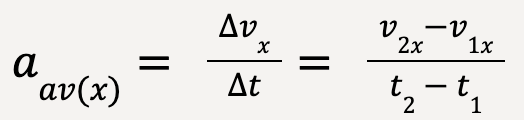
Direction of Average Acceleration
Scenario 1: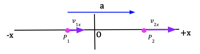 Figure 11: The initial velocity vector, v1x is in the positive x-direction. The final velocity vector, v2x is larger in magnitude and in positive x-direction. The initial velocity of the particle is positive and it became more positive with time. Hence, the average acceleration is positive and particle is speeding up in +x-direction. | Scenario 2: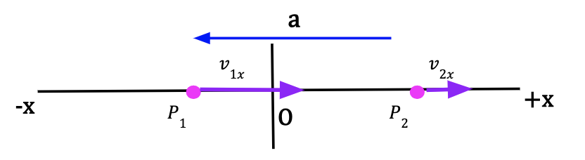 Figure 12: The initial velocity vector, v1x is in the positive x-direction. The final velocity vector, v2x is smaller in magnitude and in positive x-direction. The initial velocity of the particle is positive and it became less positive with time. Hence, the average acceleration is negative and the particle is slowing down in the +x-direction. |
Scenario 3: Figure 13: The initial velocity vector, v1x is in the negative x-direction. The final velocity vector, v2x is larger in magnitude and in negative x-direction. The initial velocity of the particle is negative and it became more negative with time. Hence, the average acceleration is negative and particle is speeding up in -x-direction. | Scenario 4: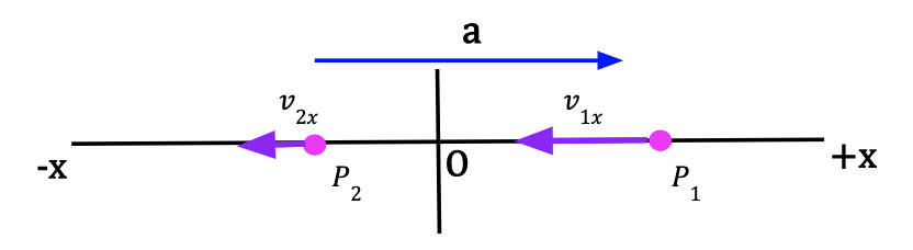 Figure 14: The initial velocity vector, v1x is in the negative x-direction. The final velocity vector, v2x is smaller in magnitude and in negative x-direction. The initial velocity of the particle is negative and it became less negative with time. Hence, the average acceleration is positive and particle is slowing down in the -x-direction. |
The direction of the average acceleration vector is along the direction of the initial velocity vector (v1x) if the particle is speeding up between points P1 and P2, and it is opposite to the direction of the initial velocity vector (v1x) if the particle is slowing down between points P1 and P2.
Why do we look at the direction of initial velocity vector when identifying whether the average acceleration is positive or negative?
Consider a particle at point P1 moving along the x-axis with a positive x-velocity, v1x. After some time, the particle is at point P2 and the particle’s x-velocity is now negative. Since the particle’s initial x-velocity is positive and it became less positive, we can conclude that the average acceleration is negative and particle is now speeding up in the negative x-direction. At P2, the acceleration is in the same direction as the particle’s velocity at P2.
The particle’s initial velocity is in the positive x-direction while the acceleration is negative. The particle starts to slow down in the positive x-direction, momentarily comes to a stop and finally, the particle reverses its direction and starts speeding up along the negative x-direction (see below).

Graphical Representation
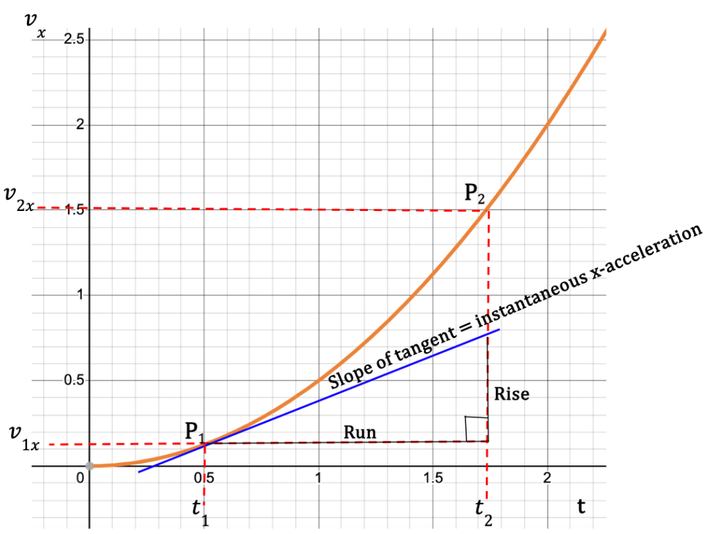
When a particle’s x-velocity is graphed with respect to time, the slope of the line between points P1 and P2 is equivalent to the average acceleration in the x-direction.
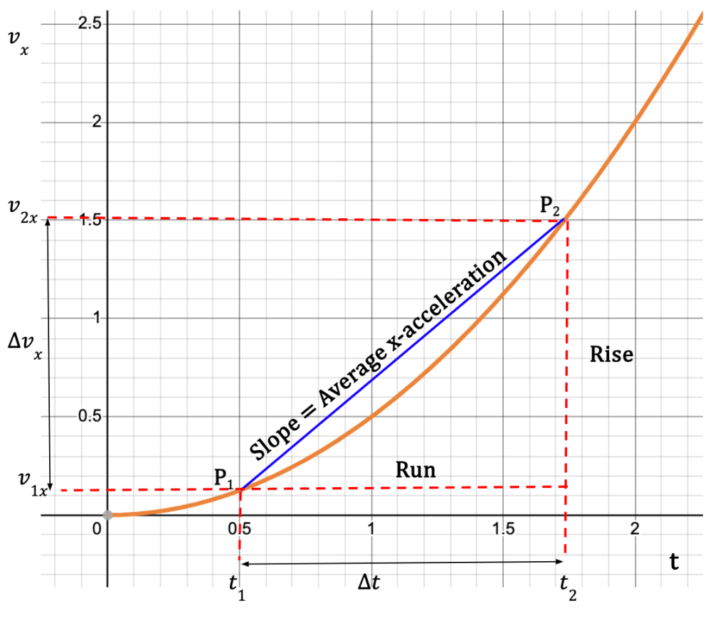
Figure 16: The vx-t curve provides the change in particle’s velocity with respect to time. At point P1, the particle has an x-velocity, v1x and at point P2, the x-velocity is given by v2x. The slope of the graph is equal to the average x-acceleration which is given by Δvx/Δt.
Scenario 1 (Positive Slope)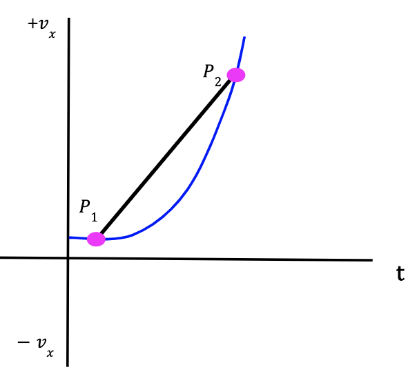 Figure 17: At P1, velocity is positive and it becomes more positive with time. We can conclude that the average acceleration between points P1 and P2 is positive and particle is speeding up in the +x-direction. This can be confirmed by the direction of the slope which is positive. | Scenario 2 (Positive (Slope)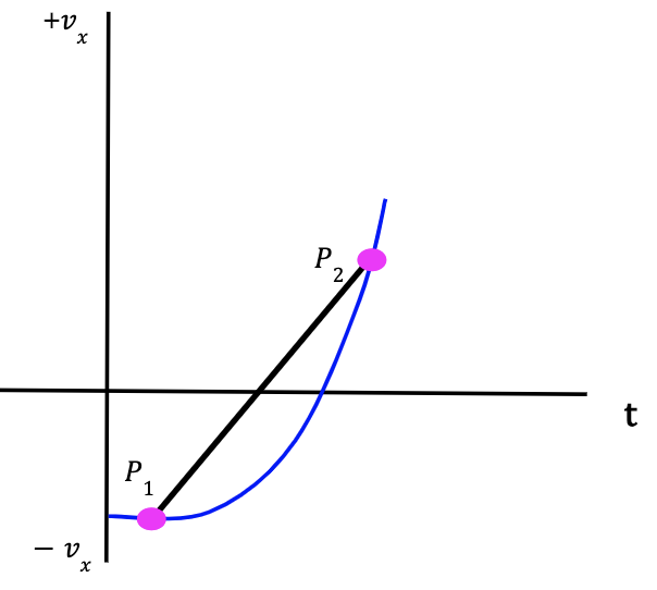 Figure 18: At P1, velocity is negative and it becomes less negative with time. We can conclude that the average acceleration between points P1 and P2 is positive and particle slowed down in the -x-direction and then started speeding up in the +x-direction. |
Scenario 3 (Negative Slope)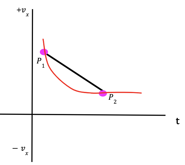 Figure 19: At P1, velocity is positive and it becomes less positive with time. We can conclude that the average acceleration between points P1 and P2 is negative and particle slowed down in the +x-direction. | Scenario 4 (Negative Slope)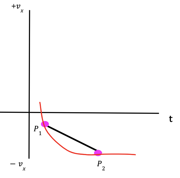 Figure 20: At P1, velocity is negative and it becomes more negative with time. We can conclude that the average acceleration between points P1 and P2 is negative and particle speeding up in the -x-direction. |
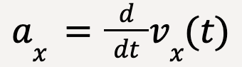
Instantaneous Acceleration
If in Figure 16, we start moving P2 closer to P1 such that Δvx and Δt become infinitesimally small, the instantaneous x-acceleration is given by the average x-acceleration in the limit that Δt approaches zero, which is also called the derivative of vx with respect to t.
 ……(7)
……(7)
Remember, ax is the component of instantaneous acceleration in the x direction (See Error #2).
Graphical Representation
Vx-t Graph
The graph of instantaneous velocity (vx) with respect to time (t) is called a vx-t graph.
On a vx-t graph, the instantaneous x-acceleration at a point is equal to the slope of the tangent to the curve at that point.
The Slope
If the slope of the tangent is positive, the direction of instantaneous acceleration is positive. In the other words, the acceleration is towards the positive x-axis. Conversely, if the slope of the tangent is negative, the direction of instantaneous acceleration is negative or its towards the negative x-direction.
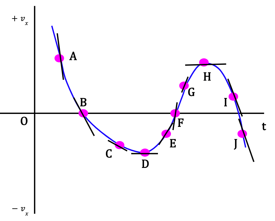
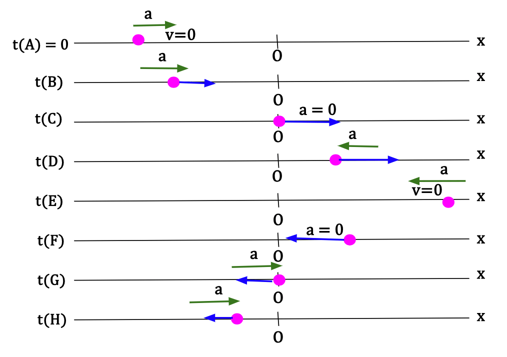
At point A
Velocity is positive which means that the particle is moving in +x-direction and the velocity is getting less positive with time. The slope of the tangent drawn at this point is negative which means that acceleration is directed towards the negative x-direction. Since velocity and acceleration are in opposite direction, particle is slowing down as it moves alongs the positive x-axis.
At point B
The velocity of the particle is zero but acceleration is not. The slope of the tangent drawn at this point is negative and thus, acceleration is towards the negative x-direction. The particle at this point is momentarily at rest and will start speeding up in the negative x-direction.
At point C
The acceleration is still in the negative x-direction since the slope is negative, but compared to points A and B, the slope is not as steep, which means that the magnitude of acceleration dropped leading to a reduced rate of change in velocity. In other words, velocity at point C is not changing as rapidly as points A and B. The velocity at point C is negative. Since velocity and acceleration are in the same direction, particle is accelerating in the negative x-direction.
At point D
The slope of the tangent to the curve is zero which means that acceleration is zero. The velocity of the particle is momentarily constant and directed towards the negative x-direction.
At point E
Velocity is in the negative x-direction. The slope of the tangent to the curve is positive which means that acceleration is now directed towards the positive x-direction. Since velocity and acceleration have opposite signs, the particle is slowing down as it moves along the negative x-direction.
At point F
The velocity of the particle is zero but the acceleration is a positive non-zero quantity given that the slope is positive. This means that the particle is momentarily at rest and will start speeding up in the positive x-direction.
At point G
The velocity of the particle is positive. The acceleration of the particle is also positive which means that the particle is speeding up in the positive x-direction. However, the strength of acceleration at point G is not as large as at point F because the slope is comparatively less steep. This means that the velocity is changing less rapidly at point G when compared to point F.
At point H
The slope of the tangent to the curve is zero which means that acceleration is zero. The velocity is positive and momentarily constant at this point.
At point I
Velocity of the particle is positive which means that it is moving in the positive x-direction. However, the slope of the tangent is negative which means that acceleration is directed in the negative x-direction. Since, velocity and acceleration are in opposite directions, the particle is slowing down as it moves along the positive x-direction.
At point J
The velocity of the particle is negative. Due to a negative slope, the acceleration is also towards the negative direction which means that the particle is speeding up in the negative x-direction.
Figure 22: vx-t curve is represented in blue with black lines for tangents to the curve at points given in pink. Click on the black triangles for more information8.
X-t Graph
Information about the acceleration can also be drawn from an x-t graph. This is because instantaneous acceleration (ax) is equal to the second derivative of position (x) with respect to time (t),
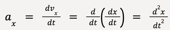 …..(8)
The curvature of an x-t curve at a point gives information about acceleration at that point. If the function is curved up (or concave up), acceleration is positive. If instead, the function is curved down (or concave down), acceleration is negative. If the function at the point is straight with no curvature, acceleration is zero and velocity is constant. This is true for second derivative of any function. Greater is the curvature of the function, larger is the magnitude of acceleration9.

At point A
The particle is somewhere on the negative x-axis. The slope of the tangent at this point is zero which means that velocity of the particle is zero and it is momentarily at rest. The function is curved upwards which means that acceleration at this point is positive and the particle will start moving in the positive x-direction.
At point B
The particle is on the negative x-axis with a velocity that is pointed towards the positive x-axis because the slope is positive. The function at this point is curved up which means that acceleration is positive. Since velocity and acceleration are in the same direction, this means that the particle is speeding up along the positive x-direction.
At point C
Particle returns to the origin and has a positive velocity because the slope is positive. The function at this point has no curvature which means that acceleration is zero and the particle is moving with a constant velocity.
At point D
The particle is now on the positive x-axis. It has a positive velocity because the slope is positive. The function is slightly curved downwards suggesting that the acceleration is in the negative direction and has a small magnitude. Since velocity and acceleration are in the opposite direction, this means that the particle is slowing down as it moves along the positive x-axis.
At point E
The particle is on the positive x-axis. The slope is zero which means that the velocity is zero. The function is curved downwards which means that acceleration is negative. The particle is momentarily at rest and will start to move in the negative x-direction.
At point F
The particle is on the positive x-axis. The slope is negative which means that the velocity is in the negative x-direction. The function has no curvature at this point which means that acceleration is zero. The velocity of the particle is momentarily constant.
At point G
The particle again returns to the origin. The velocity of the particle is in the negative x-direction because the slope is negative. The function is curved upwards which means that the acceleration is positive. Since velocity and acceleration are in opposite directions, particle is slowing down in the negative x-direction.
At point H
The particle is now on the negative x-axis. Velocity is negative because the slope is negative. Compared to magnitude of velocity at point G, the magnitude at point H is smaller because the slope is not as steep. The function is still curved up meaning that the acceleration is pointed towards the positive x-direction. Since velocity and acceleration have opposite signs, particle is slowing down as it moves along the negative x-direction.
Figure 23: The x-t curve is shown in purple with tangents drawn with black at points given in pink. Click on the black triangles for more information.
Motion Diagram
A motion diagram, as discussed previously, can be created for Figure 23.
Motion with Constant Acceleration (Young et al., 2016)
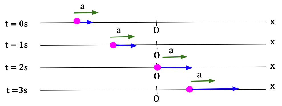
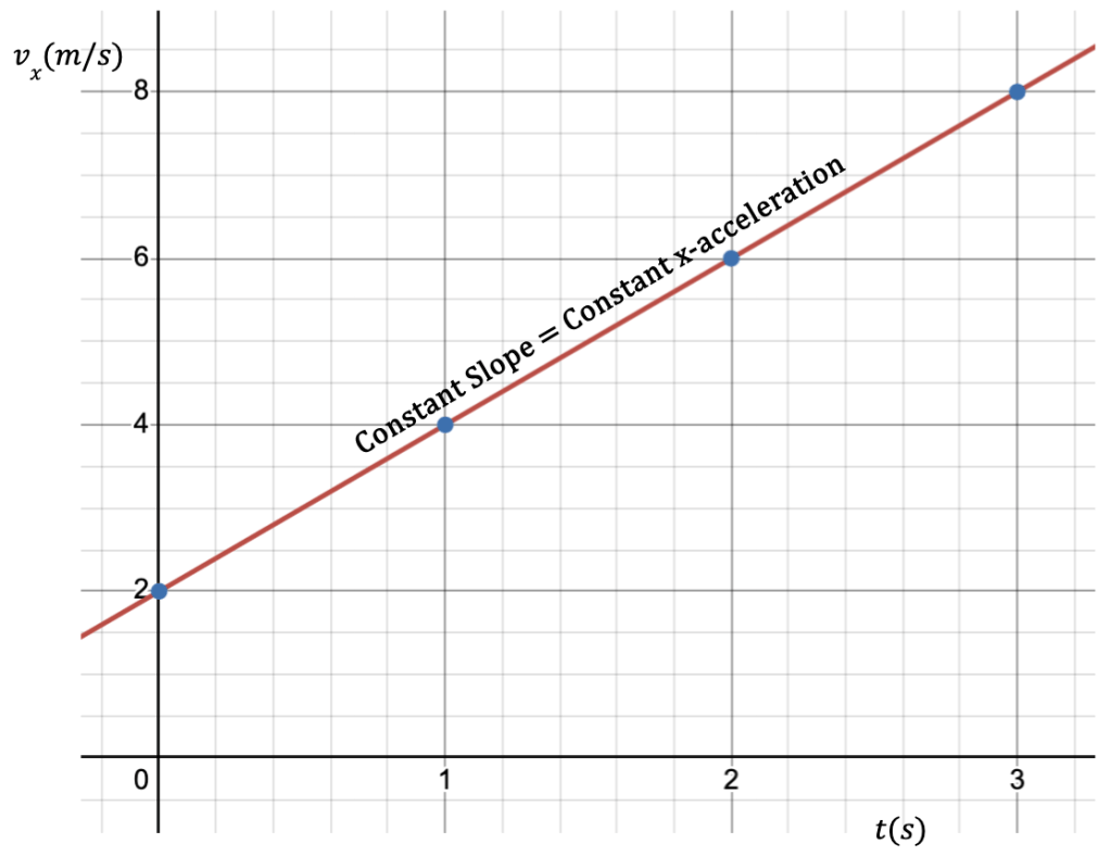
A particle moving with constant acceleration means that the velocity of the particle is changing by an equal amount over each time interval which is held constant.
Consider a particle starting with a velocity, vx = 2 m/s at t = 0 s. The time interval, Δt, is held constant and taken to be 1s. The subsequent changes in velocity are shown in the following table:
| t | vx |
|---|---|
| 0 | 2 |
| 1 | 4 |
| 2 | 6 |
| 3 | 8 |
For t1 = 0 s and t2 = 1 s, Δt = 1 s and Δvx = (4 -2) m/s = 2 m/s
aav(x) = Δv/Δt = 2 m/s2
For t1 = 1 s and t2 = 2 s, Δt = 1 s and Δvx = (6 -4) m/s = 2 m/s
aav(x) = Δv/Δt = 2 m/s2
For t1 = 2 s and t2 = 3 s, Δt = 1 s and Δvx = (8 -6) m/s = 2 m/s
aav(x) = Δv/Δt = 2 m/s2
Velocity over a time interval Δt = 1 s changes at a fixed rate giving an acceleration that is constant. In other words, velocity is increasing by 2 m/s every second.
Particle’s motion can be shown on a motion diagram as follows:
For constant acceleration, average acceleration over any time interval is equal to the instantaneous acceleration at any point along the x-axis. This means that,
 …..(9)
Let the time interval start at time t1 = 0 with an initial velocity, v0x. Then at time t2 = t, the velocity of the particle is given by vx.
 ……(10)
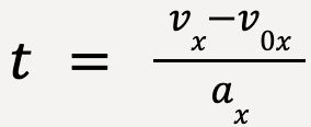
Rearranging equation 10, the final velocity of the particle is given by;
 ……(11)
The final velocity of the particle is equal to the sum of initial velocity, v0x and the product of x-acceleration with time interval, t. In other words, the change in x-velocity, vx – v0x is equal to axt.
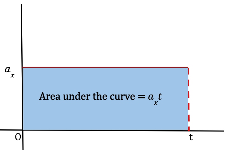
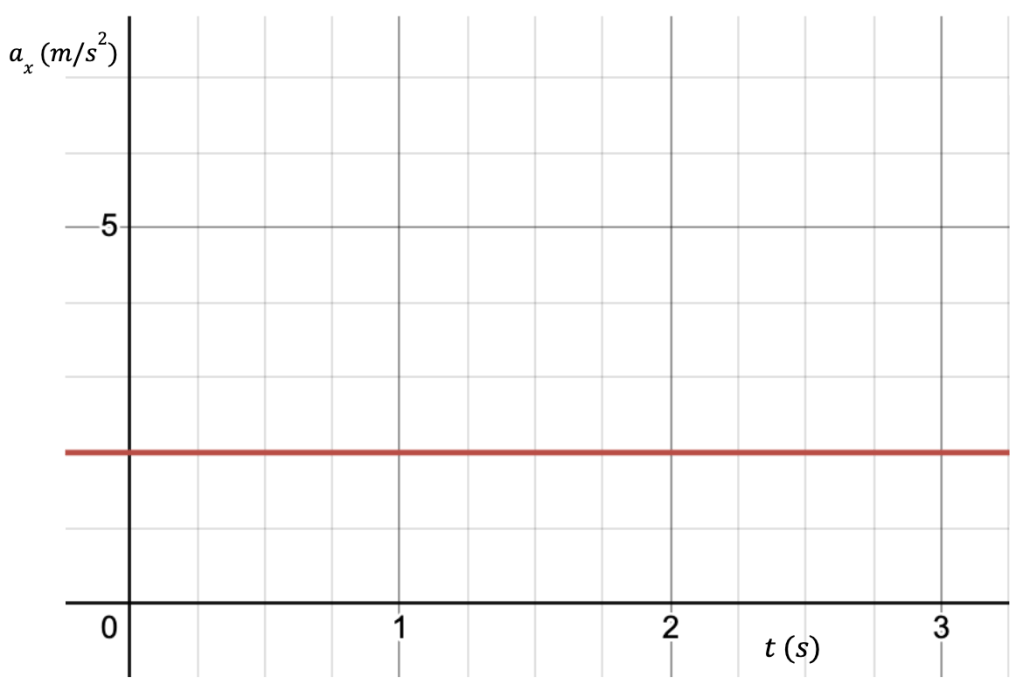
Figure 28: If we look at the ax-t graph for constant acceleration, ax over time interval t, we notice that the area under the curve is equal to the area of a rectangle (shaded blue region) with sides ax and t. The area of this rectangle is equal to axt.
This means that the change in x-velocity, vx – v0x is equal to the area under the curve between the time interval on an ax-t graph.
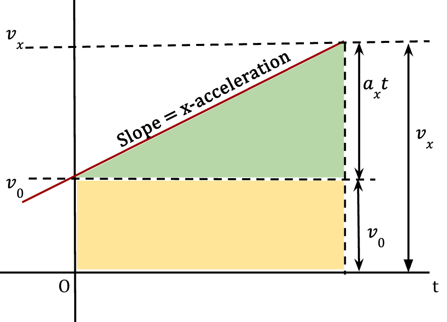
Figure 29: On a vx – t graph, the area under the straight line is equal to the area of the green triangle and the area of the yellow rectangle. The height of the triangle is equal to axt12 because as discussed earlier, vx – v0 = axt. Area of ∆ = 1/2*t*axt = 1/2*ax*t2. The area of rectangle is equal to v0*t. The total area under the straight line is then equal to v0t + 1/2axt2.
Similarly, an equation can be derived for the position, x of the particle when acceleration, ax is constant.
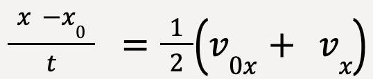
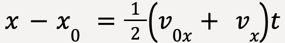
As discussed in equation 3, the average velocity of a particle over a time interval, Δt is given by,
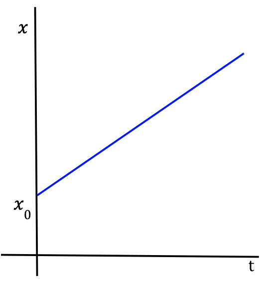
Let the particle at t1 = 0 be at position x1 = x0. After some time, at t2 = t, the particle is located at x2 = x. The average x-velocity is given by;
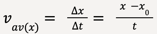 …..(12)
Note: Equation 12 is true regardless of whether the acceleration is constant or not.
The average velocity, vav(x) is also equal to the average of the initial and final velocity,
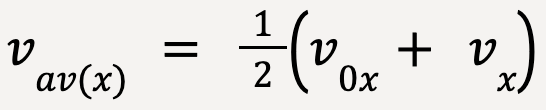 …..(13)
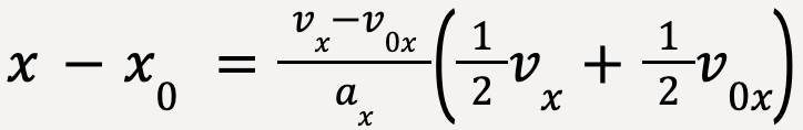
Note: This expression is true only because acceleration is constant and velocity is increasing with a steady rate.
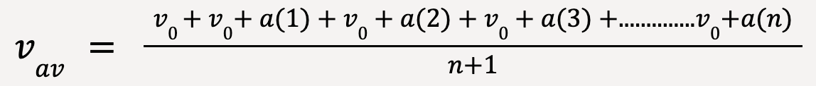
Proof
Consider a particle with initial velocity, v0 at time, t0 = 0. Given that the acceleration, a, is constant, an expression for the final velocity, v can be derived using equation 11;
v = v0 + at…..(14)
where t = 1, 2, 3, 4, 5,………., n.
The average velocity for Δt = n-0 = n, can be calculated as follows;
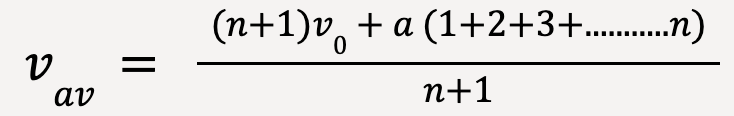
The sum of n-numbers is given by, 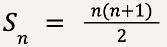
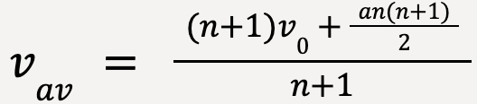

Therefore, the average velocity, vav is equal to the average of initial velocity, v0 and final velocity, v0 +an.
Equating equations 12 and 13,
which gives,
 …..(14)
Equation 14 is applicable to use when it is known that acceleration is constant but the value is not given.
Using equation 11, vx = v0x + axt;
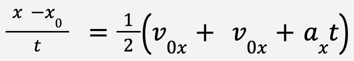

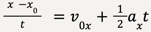
 ……(15)
 ……(16)
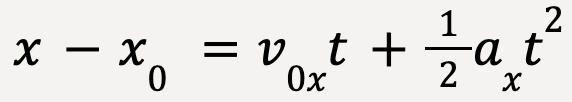
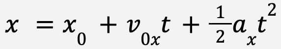
If in equation 16, the acceleration is zero, x = x0 + v0xt, which means that the displacement of the particle when velocity is constant is given by the product of velocity and time (v0xt).
This means that when acceleration is not zero, the position of a particle, x is equal to the sum of:
- x0: The initial location along the x-axis
- v0xt: The displacement of the particle if acceleration was zero and velocity was constant
- (1/2)axt2: The displacement of the particle due to change in velocity caused by a non-zero acceleration
Comparing equation 15 to Figure 29, we can see that for constant acceleration, the area under the straight line on a vx-t graph is equal to the change in position or displacement of the particle (x-x0).
Note: The area under the ax-t curve between the given time interval is always equal to the change in velocity even if acceleration is not constant. However, in that case, v – v0x would not necessarily equal axt. Similarly, the area under the vx-t curve between the given time interval always gives the change in position of the particle even if acceleration is not constant. However, equation 16 would no longer apply.
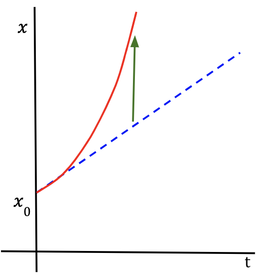
Since equation 16 is quadratic because the degree (highest power of the variable, t) is equal to two, the x-t graph for constant acceleration will always be a parabola.
To understand why the graph is a parabola for constant acceleration, consider the x-t graph for a particle with zero x-acceleration which means that it is moving with a constant velocity.

Finally, an equation of motion for constant acceleration that does not include time can be derived from equations discussed earlier.
This can be done by substituting the value of t given by equation 11 into equation 16;
Plugging the value of t into equation 16:
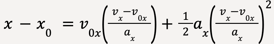
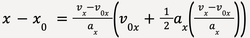
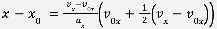
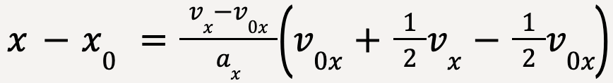

Using the algebraic identity (a+b)(a-b) = a2-b2,
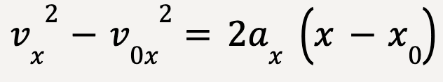
or
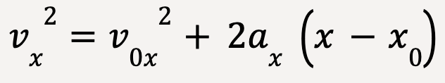 …..(17)
Equations 11, 14, 16 and 17 are defined as the equations of motion with constant acceleration. Every single problem that includes straight line motion with constant acceleration can be solved using these equations.
Equations of Motion with Constant Acceleration
-
- vx is the final velocity of the particle at t = t
- v0x is the initial velocity of the particle at t=0
- ax is the value of constant acceleration
- t is the time taken by the particle’s motion starting at t=0
-
- x is the final position of the particle at t=t
- x0 is the initial position of the particle at t=0
- v0x is the initial velocity of the particle at t=0
- vx is the final velocity of the particle at t=t
- t is the time taken by the particle’s motion starting at t=0
-
- x is the final position of the particle at t=t
- x0 is the initial position of the particle at t=0
- v0x is the initial velocity of the particle at t=0
- t is the time taken by the particle’s motion starting at t=0
- ax is the value of constant acceleration
-
- vx is the final velocity of the particle at t=t
- v0x is the initial velocity of the particle at t=0
- ax is the value of constant acceleration
- x is the final position of the particle at t=t
- x0 is the initial position of the particle at t=0
Free Falling Bodies (Young et al., 2016)
The most popular example of straight line motion with constant acceleration is that of a body falling under the force of gravity, commonly described to be in free fall. As theorized by Galileo, all bodies fall with a constant acceleration regardless of how much they weigh. This statement is true as long as air resistance is negligible.
Note: Acceleration of a falling body is constant with following assumptions:
- Air resistance is negligible
- Distance that the body falls is comparatively much smaller than the radius of the Earth
- Effects of Earth’s rotation are negligible
This constant acceleration is referred to as acceleration due to gravity and is usually taken to be g = 9.80m/s2.
Motion when Acceleration is not Constant (Young et al., 2016)
Velocity and Acceleration by differentiation
If acceleration is not constant,
Velocity can be determined from the position function13, x(t), using:
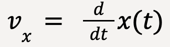 ….(18)
X-velocity is the derivative of position function with respect to time.
Similarly, x-acceleration can be determined from the x-velocity function, vx(t) using:
 ….(19)
X-acceleration is the derivative of x-velocity with respect to time.
Velocity and Position by Integration
When only the acceleration function is known, velocity and position functions can be derived using calculus, specifically, by the method of integration.
Consider a function of acceleration which varies with time, given by, ax(t). If the time interval from t1 to t2 is split into equal mini-intervals of Δt and aav(x) is the average acceleration for this time interval, Δt (as shown in Figure 34), then according to the definition of average acceleration;
or
 ….(20)
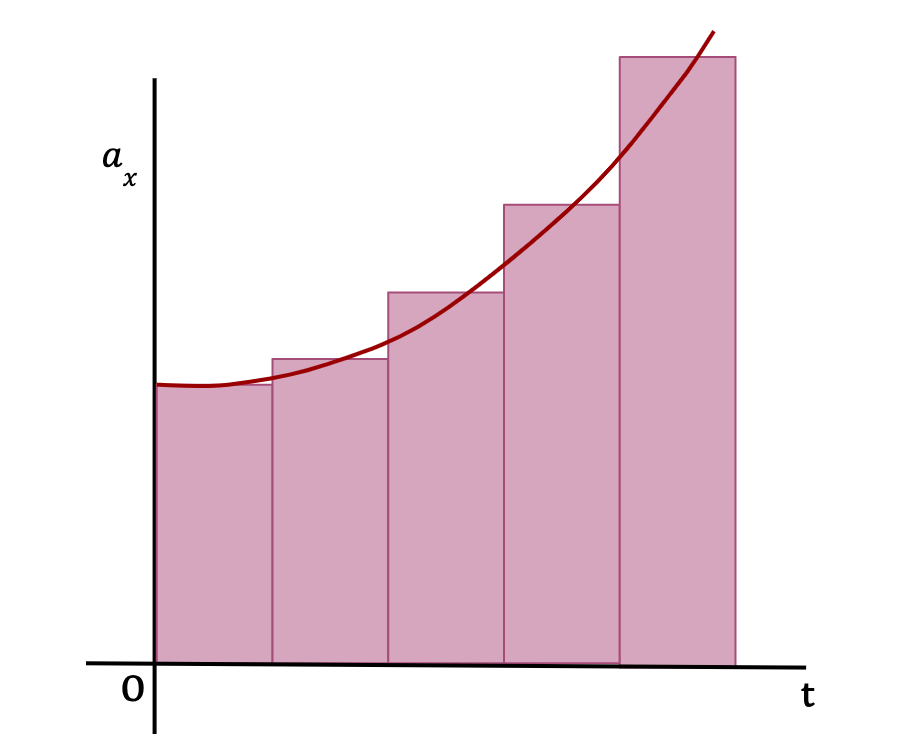
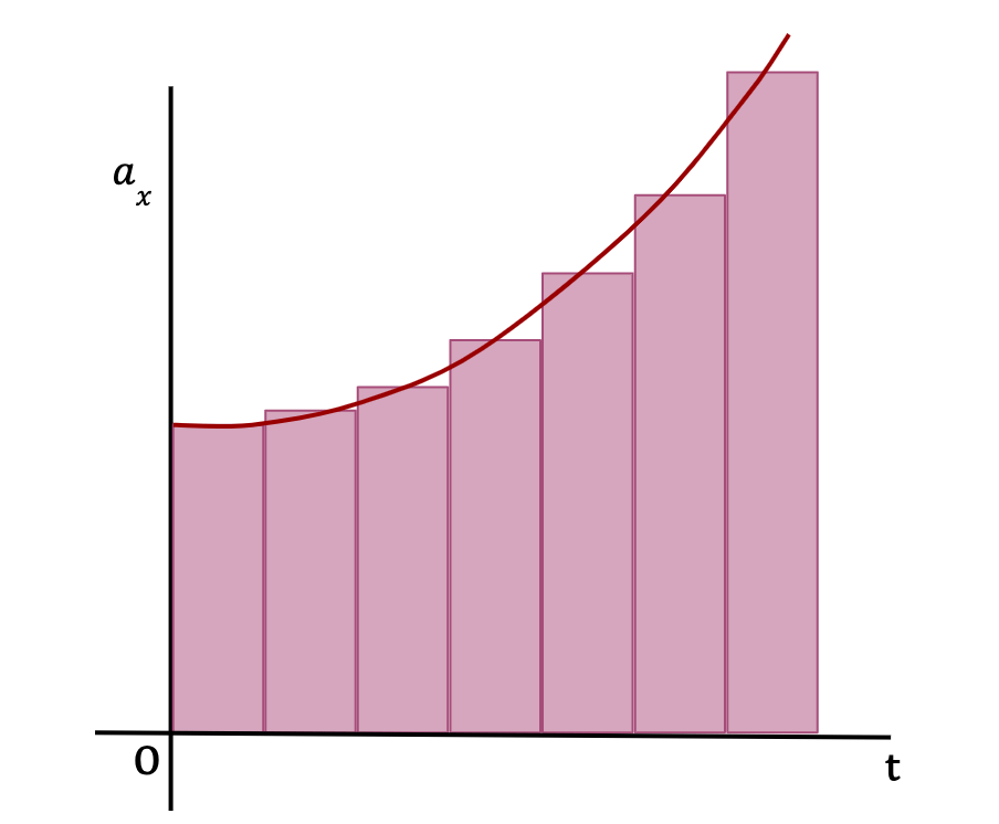
The change in x-velocity of the particle over the time interval Δt is equal to the product of the average x-acceleration and the time interval Δt. This means that the change in x-velocity is also equal to the area of the rectangle (as shown in Figure 34) which approximately equals the area under the curve between the given time interval, Δt.
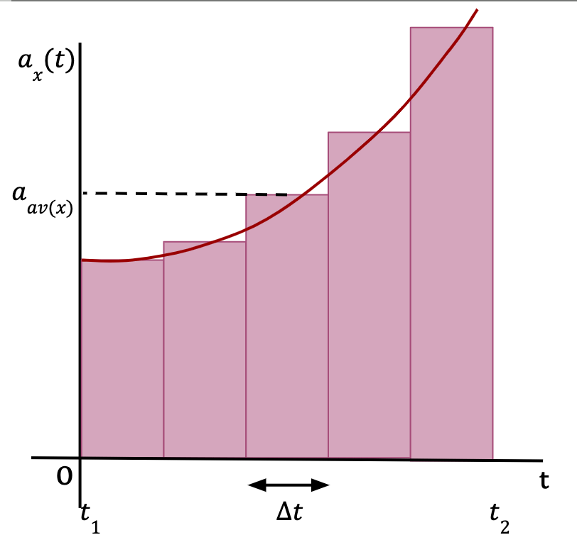
The total change in x-velocity of the particle between times t1 and t2 (ΔVx) is then equal to the sum of changes in x-velocity over each time interval Δt, which is approximately equal to the total area under the curve on an ax-t graph (see Figure 34). In other words;
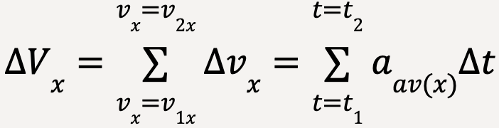 …..(21)
As Δt becomes really small and number of Δt’s become very large, the area of the rectangles approaches the area under the graph (See below). In other words, the average x-acceleration from any time t to t+Δt approaches the instantaneous x-acceleration, ax(t) at time t.
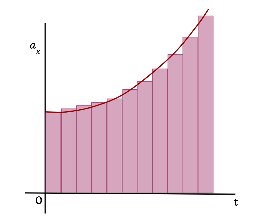


In the limit that Δt becomes negligible and the number of Δt’s become infinite, the area under the curve is equal to the integral of instantaneous x-acceleration from t1 to t2. In other words,
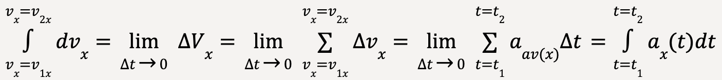
The change in x-velocity of the particle is equal to the time integral of x-acceleration;
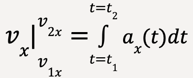
 ….(22)
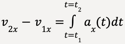
If the initial velocity of the particle at t1 = 0 is v0x and the final velocity at t2=t is vx ;
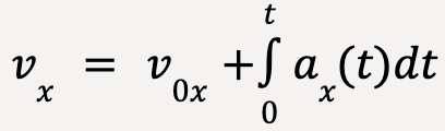 ….(23)
Similarly, the same procedure can be applied to a vx-t graph such that change in the position (or displacement) of the particle is equal to the time integral of the x-velocity;
 ….(24)
The change in the position of the particle can then be written as;
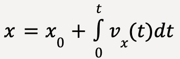 ….(25)
where x0 is the initial position of the particle at t1 = 0 and x is the final position of the particle at t2 = t.
To summarize, the instantaneous velocity of the particle, vx can be determined using equation 23 when acceleration is given as a function of time, ax(t), and the initial velocity of the particle, v0x is known. Once the velocity of the particle has been deduced, it can be used to determine the position, x, of the particle using equation 25 given that the initial position of the particle, x0, is known.
Common Errors in Understanding (Young et al., 2016)
Error #1:
Speed and Velocity are two different quantities. Speed is a scalar quantity which is given by distance travelled divided by the time taken. On the other hand, velocity is a vector quantity and is given by the particle’s displacement divided by the time interval.
The magnitude of average velocity is not the same as average speed.

Consider a beam bridge of length 20.0 m. You walk from one end of the bridge to the other and then walk back to the point where you started. The round trip takes you half a minute to complete. Your average speed is distance/time = (20+20)m/30s = 1.33 m/s. However, your displacement for the whole trip is zero and thus, the magnitude of average velocity will be zero.
However, magnitude of instantaneous velocity is the same as instantaneous speed. At a certain instant, instantaneous speed tells you how fast a particle is moving while instantaneous velocity tells you how fast and in what direction the particle is moving.
Back to Instantaneous Velocity
Error #2:
Whether the particle is speeding up or slowing down cannot be determined from the algebraic sign of instantaneous x-acceleration. Both instantaneous x-velocity and instantaneous x-acceleration need to be considered to find out about the particle’s speed. If vx and ax are in the same direction, particle is speeding up and if vx and ax are in the opposite direction, particle is slowing down.

Back to Instantaneous Acceleration
- Young, H.D. et al. (2016) Sears and Zemansky’s university physics: With modern physics. 14th edn. Boston: Pearson. ↩︎
- Δx is not to be confused as the product between Δ and x. Δ is a symbol commonly used to describe change in a given quantity, whereby the change is equal to final value – initial value (not initial – final). ↩︎
- Refrain from saying that since the particle moves to the right, displacement vector is in the positive direction. One could chose to have the -x direction pointed towards the right, in which case displacement vector will be negative if it is pointing towards the right. ↩︎
- Change in time will always be positive because you can only move forward in time. ↩︎
- The orange curve should not be mistaken to be the path taken by the particle, which is a straight line (yellow vector on the left). The curve represents the change in the particle’s position with respect to time. ↩︎
- A particle can have a positive location (+x-coordinate) and have negative average or instantaneous velocity. The direction of average or instantaneous velocity does not depend on the location of the particle but instead depends on the change in it’s location (whether the change is along positive or negative x-axis). ↩︎
- If the point is above the origin, it is located on the positive x-axis and if the point is somewhere below the origin, it is located on the negative x-axis. ↩︎
- Instantaneous x-acceleration is referred to as simply ‘acceleration’ and instantaneous x-velocity is referred to as simply ‘velocity’. ↩︎
- Numerical value of acceleration is hard to determine from an x-t curve because curvature cannot be measured easily. ↩︎
- For constant acceleration, average and instantaneous acceleration will be the same. ↩︎
- Graph of x-acceleration with respect to time is called an ax-t graph. ↩︎
- Alternatively, slope = rise/run = axt/t = ax which makes sense because the slope of the line should equal the x-acceleration of the particle. ↩︎
- Position is given as a function of time. ↩︎
